Conditional Formatting in Google Sheets: Comprehensive Guide with Examples

In this article, we’ll explain how to make conditional formatting in Google Sheets with step-by-step guide. Also, you will find many different conditional formatting Google Sheets examples with images and clear instructions.

Table Of Content

1. Conditional Formatting in Google Sheets
2. How to do Conditional Formatting in Google Sheets?
3. Conditional Formatting Examples
4. Out-of-Box Examples of Conditional Formatting in Google Sheets
5. How to copy and paste conditional formatting to another Google Sheet?
6. How to delete a conditional formatting rule in Google Sheets?
7. Conclusion

The purpose of this blog post is to underline the nuances of Google Sheets conditional formatting. By the end, you will be able to add visually striking and educational conditional formats to your spreadsheets.

1. Conditional Formatting in Google Sheets

Google Sheets is a very adaptable and user-friendly tool in the ever changing field of data analysis and presentation. Conditional formatting is a particularly useful feature of Google Sheets. It lets users apply particular formatting to cells based on predefined criteria.

What are the key components of Google Sheets conditional formatting?

Firstly, we’ll try to explain the key components of conditional formatting to better understand how it works.

• Range: The spreadsheet cells to which the conditional formatting rule will be applied are referred to here.
• Condition: This is the criteria that determine whether the formatting should be applied to a cell within the range.
• Formatting: The specific visual changes (like color, font style) that will be applied to the cells that meet the condition.

Thus, we can set up any rule-based formatting styles by using these three elements.

Besides, it’s worth underlying that Google Sheets gives us two options to apply stylings:

1. Color Scale
2. Single Color

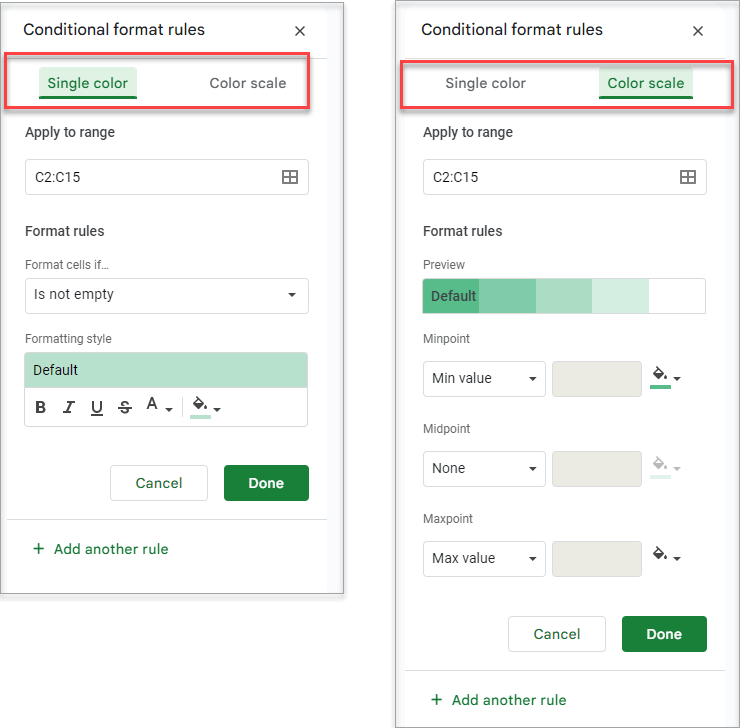
While the color scale option gives a color map according to the cell values in the selected range, the single color option makes cell-based formatting.

Let’s see how to apply conditional formatting Google Sheets rules.

2. How to do Conditional Formatting in Google Sheets?

Now, we’ll basically explain the main steps to add conditional formatting rules in Google Sheets.

Step 1: Select your range and open conditional format box

Firstly, you should highlight or select the range that you want to apply conditional formatting rules. Alternatively, you can directly open the conditional format box and write your range on that box:

Go to Format > Conditional Formatting from the top menu, and then there will open a box on the right-side of your spreadsheet, where you’ll be able to configure all your format settings.

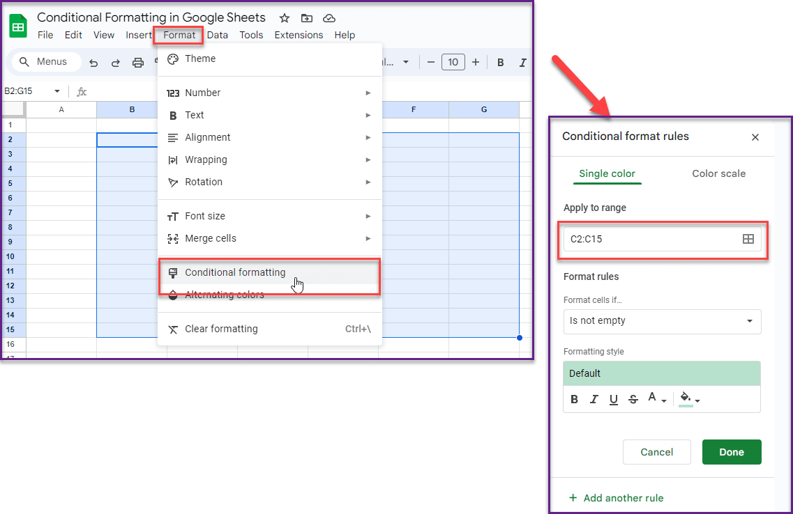
Step 2: Define Format Rules

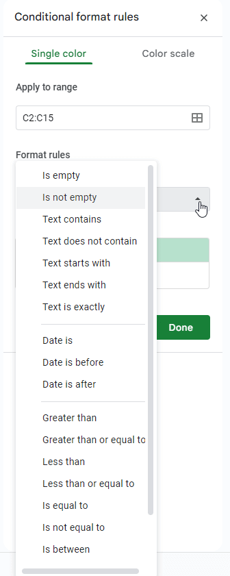
Secondly, we’ll define our criteria for the specific formats. So, Google Sheets gives you a list of different rule types including but not limited to Is empty/Is not empty, Text contains, Date is, Greater than, etc. Also, you will see a Custom Formula Is option in the end of the list. That option will let us set complex criteria, which we’ll explain with examples in the following paragraphs.

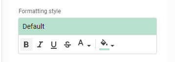
Step 3: Define your formatting style

Lastly, we’ll set up our formatting style for the selected range that meets our criteria. Therefore, you can set font color, cell color, background, font type, and other formatting styles here.

That’s how the conditional formatting works in Google Sheets. Now we’ll go over examples to better understand the dynamics of this very useful feature.

3. Conditional Formatting Examples

We will try to explain the most common applications of conditional formatting here. But please remember, the conditional formatting is a very flexible feature that you can add very complex and out-of-box criteria. So, actually the limit is the sky here.

How to do color scale conditional formatting in Google Sheets?

After selecting your range, go to Format > Conditional formatting and switch to Color-Scale from the top options.

You can select one of the default scaling colors, or you can configure a custom one for your needs:

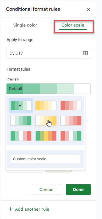
You can also play with your color ranges with Minpoint, Midpoint and also Maxpoint values and colors.

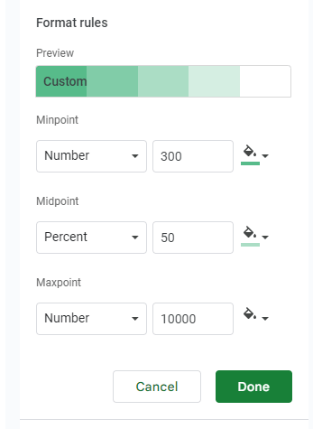
For example, we have a list of salesman and we want to make a heat map for their sales volumes. We have applied a custom formatting with changing the colors and Midpoint values. So, the results is a coloring map:

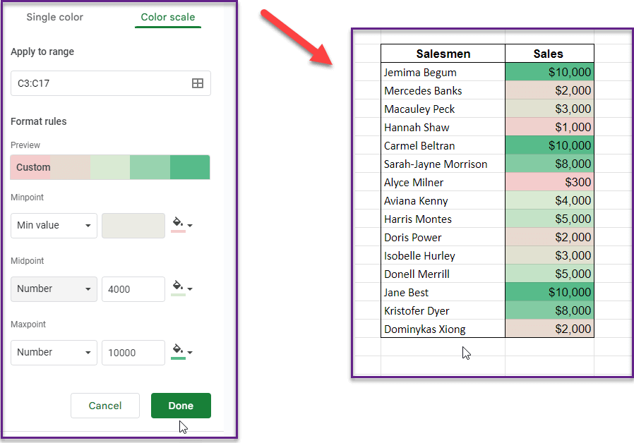
Please remember that scale coloring is a very useful and practical feature for data analysis. Because you can easily detect your underperforming and top performing or alerting values in any data set.

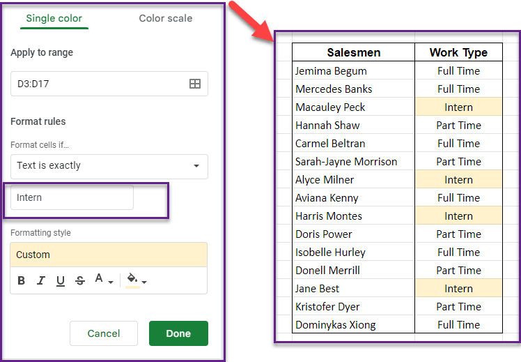
How to do conditional formatting based on text in Google Sheets?

We can add text-based criteria to our spreadsheets. This will be very useful when we want to highlight for particular texts.

First, we’ll go to Format > Conditional formatting and define our range. Then we’ll select the best option for our need.

Google Sheets gives us a list of option for text-based rules, including Empty, Not Empty, Contains, Starts and likewise rules:

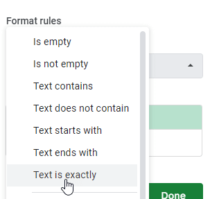
For example:

Let’s highlight the interns in our salesmen staff. We’ll use Exact text option to highlight the interns in our list:

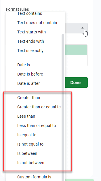
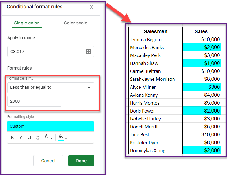
How to do conditional formatting based on numbers in Google Sheets?

Also with numbers you can add prebuilt criteria for your range.

First go to Format > Conditional formatting. After defining your range, select a defined condition from the rules list and add your limit values. Additionally, you’ll find many different condition types here including Greater, Less, Equal, Between, and so on.

For example, in the below example, we search for salesmen having sales under or equal to $2.000:

How to do conditional formatting based on date in Google Sheets?

To highlight dates that meets a specific condition:

• Select your range
• Choose ‘Date is before’ and select ‘today’ in the rules
• Set your desired formatting

For example, let’s highlight the Over Due tasks in a list:

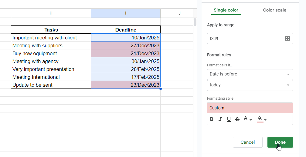
We have selected Date Before Today condition to highlight overdue tasks dynamically.

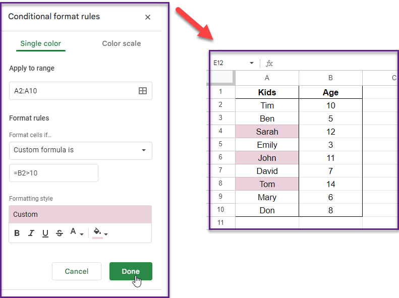
How to do Google Sheets conditional formatting based on another cell?

You can format a cell based on another cell’s value. We’ll use Custom Formula option for that.

For instance, highlighting a cell in column A if the corresponding cell in column B is greater than 10:

• Select the range in column A
• Use a custom formula like =B1>10
• Choose your formatting style

In the below example, we have highlighted the kids name whose age is greater than 10:

How to apply multiple conditional formatting rules in Google Sheets?

We can apply multiple rules by either using custom formulas or adding more than one rule.

Basically, the custom formulas offer vast flexibility. So you can give many conditions at the same time.

For example, we want to highlight the weekend in a list of days. We’ll use OR formula here to highlight both Sundays and Saturdays:

Below is the formatting result:

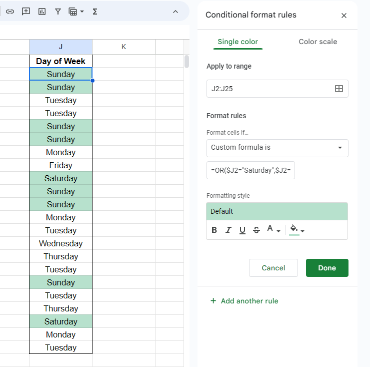
Here another important point is using the dollar signs in rule references. We should be careful about selecting the absolute cell references while configuring our format conditions.

Another option here is to add multi rules:

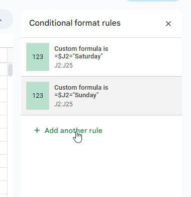
So, you can use Add another rule button to add multiple rules in Google Sheets.

4. Out-of-Box Examples of Conditional Formatting in Google Sheets

We also want to show you some out-of-box examples from Someka templates.

Our first example is from Kanban Board Google Sheets Template. The whole Kanban view here is created with conditional formatting rules. The cards colors are coming from each task’s priority, while the filters are populating the board again with font colors and background colors:

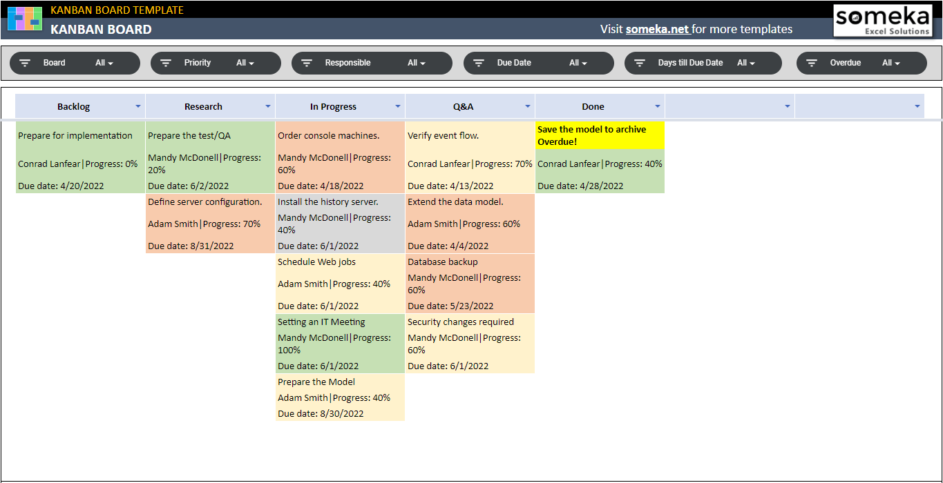
> Download Kanban Board Google Sheets Template

Also, another good example is from our Action Plan Template in Google Sheets. The navigation buttons become visible when a new goal is added to the list. So, this is another nice use of conditional formatting. By changing the font and background colors of the button cells with reference to the goal column, we create dynamic buttons:

> Download Action Plan Google Sheets Template

Then, we also want to show you an example of Work Breakdown Structure created by conditional formatting in our RACI Template. Here, all the connection lines and work structure is created by flexible rules, populating according to the filters:

> Download Responsibility Assignment Matrix Google Sheets Template

Lastly, we want to display a full dynamic form created by conditional formatting rules. In our Employee Database Google Sheets Template, we let a dynamic form creation with conditional rules:

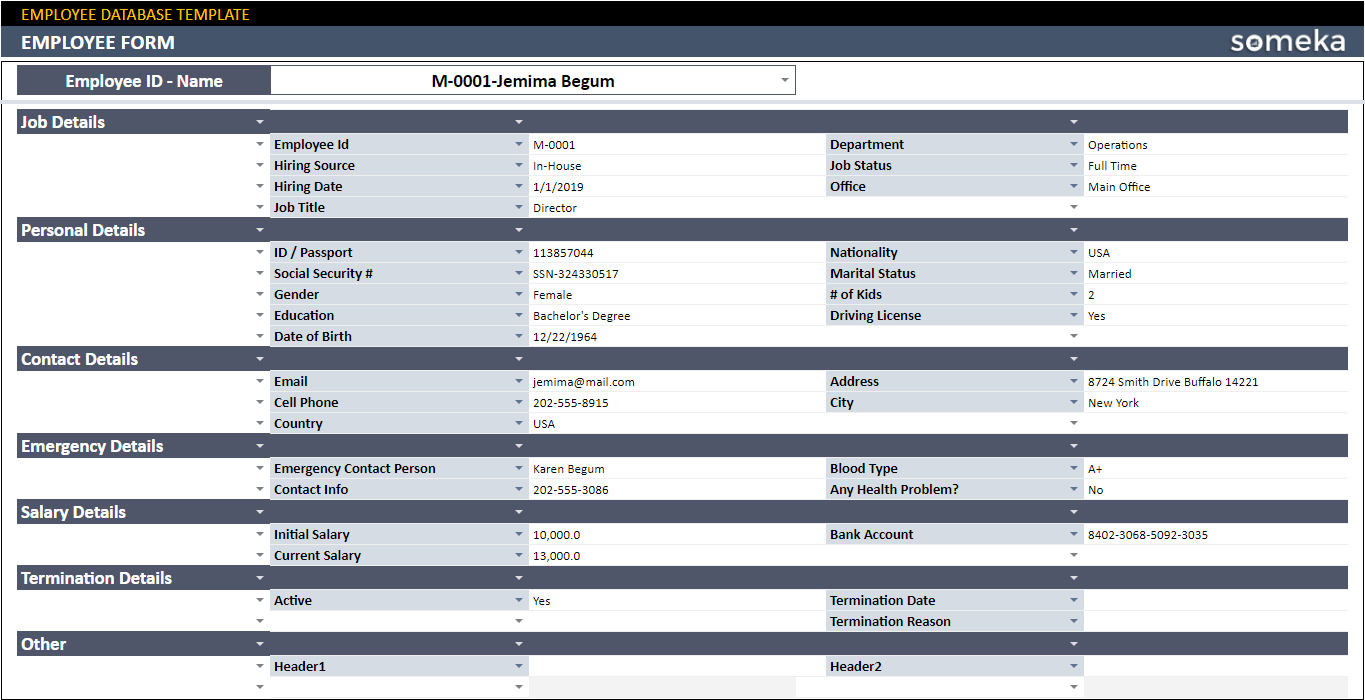
> Download Employee Database Google Sheets Template

Lastly, we want to display a full dynamic form created by conditional formatting rules. In our Employee Database Google Sheets Templates, we let a dynamic form creation with conditional rules:

In Someka portfolio, you can find hundreds of good examples of using conditional formatting rules. The ones above are some of these examples.

5. How to copy and paste conditional formatting to another Google Sheet?

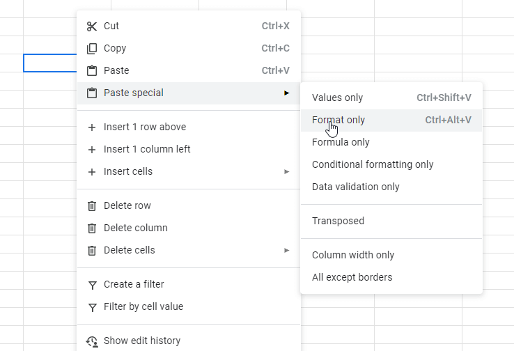
You can easily transfer a conditional formatting in a worksheet to another Google Sheets file.

To transfer formatting:

• Select the formatted cells
• Right-click and choose Copy or just click CTRL+C
• Go to the new sheet and right-click on the target range
• Select Paste special > Format Only

You can also use CTRL+Alt+V shortcut key to paste as format only.

This method is a very time-saving feature especially when you have very similar pages and do not want to add conditional rules each of them one-by-one. For example, monthly sheets or yearly financial statements might be good application area.

6. How to delete a conditional formatting rule in Google Sheets?

If you want to delete a conditional formatting rule:

• Select the range with the rule.
• Go to Format > Conditional formatting
• In the sidebar, hover over the rule and click the trash can icon to delete it.

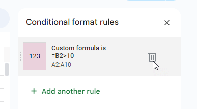
That’s how you can easily remove your conditional formatting rules.

7. Conclusion

One of Google Sheets’ most useful features, conditional formatting, can completely change the way you present data. It improves your spreadsheets’ aesthetic appeal while also making them easier to understand and analyze.

Your ability to present data will be greatly enhanced by knowing how to use conditional formatting, regardless of your level of experience.

Have fun with the formatting!

Recommended Readings:

Excel Conditional Formatting Examples – An Advanced Approach for Power Users

How to use Google Sheets as a Database? Guidance, Examples, and FAQs

How to Make a Gantt Chart in Google Sheets? Ultimate Guide