Excel Conditional Formatting Examples – An Advanced Approach for Power Users

Most spreadsheet users are familiar with the Excel Conditional Formatting feature as a data analysis tool. Finding duplicates, highlighting numbers, giving warnings are among the most common applications of this tool. But today, we’ll go a step further to introduce you some very unique and advanced usages of conditional formatting.

Table Of Content

Introduction: What can we do with Conditional Formatting in Excel?
1. Formatting Tables with Flexible Row Numbers
2. Highlighting Duplicates with Countif Formula
3. Conditional Formatting with Multi Rules
4. Tic-Tac-Toe Game with Excel Conditional Formatting
5. Other Advanced Examples
Conclusion

Let’s start!

Short Introduction: What can we do with Conditional Formatting in Excel?

In its simplest form, conditional formatting can change the color of a cell based on its value. For instance, a financial report might use red to highlight expenses that exceed a certain threshold, or blue/green to indicate profitable areas.

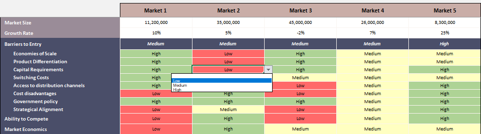
Another example, giving red, yellow and green colors for any scale of Low, Medium and High.

However, the capabilities of conditional formatting extend far beyond just color changes. It can be used to create data bars, color scales, and even icon sets that visually represent data variations. This not only enhances the readability of data but also enables users to spot trends and outliers at a glance.

1. Formatting Tables with Flexible Row Numbers

A vital aspect of conditional formatting is its dynamic nature.

Unlike static formatting, conditional rules update automatically as data changes. This means that the formatting evolves as new data is entered or existing data is modified, ensuring that the visual representation is always up-to-date.

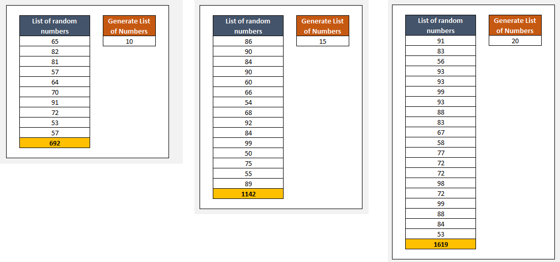
Now, let’s get into a practical application we often use in our templates. This involves dynamically formatting a list of numbers, including highlighting the total sum at the end of the list. Below examples shows a dynamic formatted list. When we change the number of items in the list from the little orange box on the left, the formatting updates automatically. Also, we have the SUM total at the bottom of each list.

This looks amazing, doesn’t it?

How to attain this flexibility?

In our example, regardless of how many numbers are generated, I always want the last row, containing the sum, to be formatted distinctly with bold and yellow text. To achieve this, we set up a formula that checks if the row number of a cell is greater than the maximum row number identified earlier.

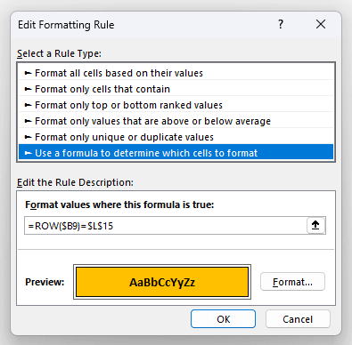
Here, it’s essential to make the row reference dynamic by removing the dollar sign from the row part of the cell reference. This adjustment allows the formula to evaluate each cell individually.

Finally, we want to eliminate borders from certain cells, which requires further adjustment of the formula.

By carefully examining the output and tweaking the formula as needed, we can ensure the formatting behaves as intended. This dynamic feature is particularly useful in dashboards and reports where real-time data monitoring is crucial.

2. Highlighting Duplicates with Countif Formula and Excel Conditional Formatting

Typically, most people use the standard ‘duplicate values’ feature for highlighting specific values, and while this works well, it has some downsides. So, we’ll demonstrate an alternative method for identifying duplicate values.

Here’s our example list:

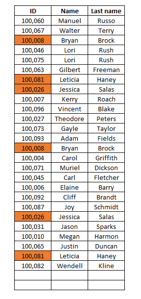
We’ll try to find duplicate ID number’s here. We can use the Standard Duplicate highlighting feature.

How to find duplicates with conditional formatting?

Go to Conditional Formatting > Duplicate Values and select the formatting type.

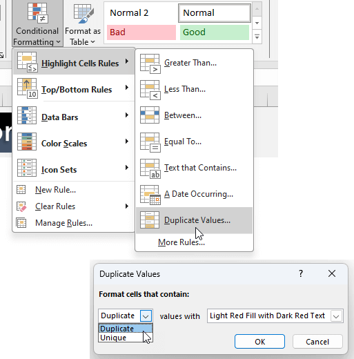
Please note that you can also highlight unique values with this method. It also allows you to make custom formats in addition to ready-made ones it offers.

Standard highlighting is pretty ok, but it will not work on the earlier versions of Excel because of comptability issues. Also, this is a pre-made method and not easy to modify. But if you have multiple criteria, then you’ll need something further.

Therefore, we often use formulas for detecting the duplicate values, which allows for more flexibility, such as comparing specific columns for duplicates.

For instance, to highlight duplicate IDs, we would utilize a COUNTIF function. This function checks if a count is higher than one, indicating a duplicate.

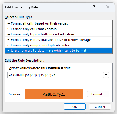
After setting up this rule, we might need to adjust the cell references to ensure the correct application of the conditional formatting.

3. Excel Conditional Formatting with Multi Rules

Furthermore, conditional formatting can be customized to suit complex criteria. Advanced rules can be set up using formulas, allowing for nuanced and specific data visualization strategies. This level of customization makes it an indispensable tool for anyone working with large datasets, from financial analysts to marketing professionals.

Let’s give an example with multi-rules. In the below table we have tasks, task status and due dates. We want to highlight the past deadlines. But we we also want that if the status of a task is Done or On Hold, we do not want any highlight.

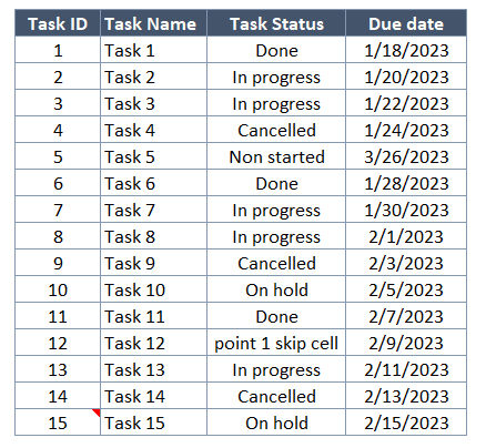
So we’ll need a complex formula here.

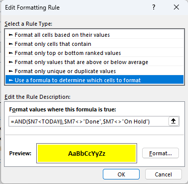
The above formula first gives a condition of the date is higher than today’s date, and then gives another condition that the next cell is not Done or On Hold. Lastly, combines these two conditions with and AND function.

4. Tic-Tac-Toe Game with Excel Conditional Formatting

Here’s another example with Tic-Tac-Toe game. We want to give red colors when any of the players manages to make a 3-item row horizontally, vertically or crosswise.

We’ll need to first make a calculation to identify 3-item sets. You can use COUNTIFS function here to make the formula. It basically checks if the count of items is equal to three and not empty, and gives “W” for WIN situation.

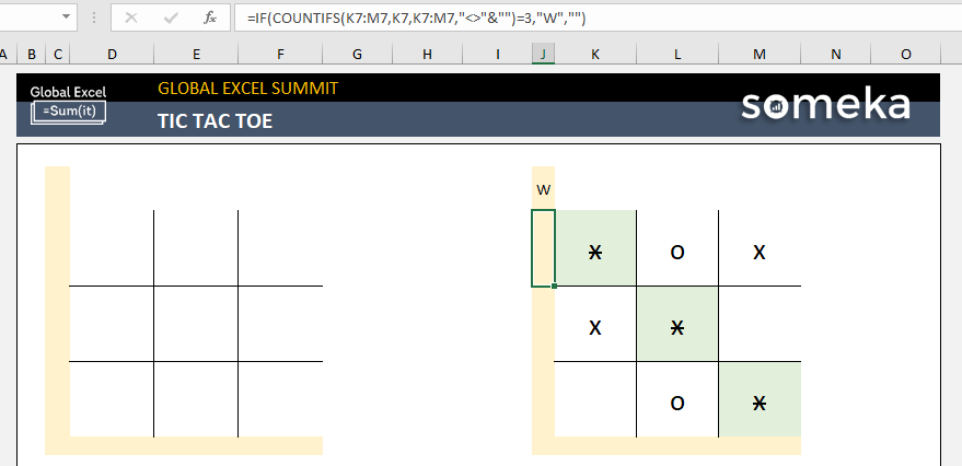
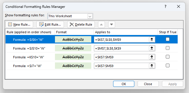
Now it’s time to use this W as the conditional formatting rule. If the starting cell equals to W, then the row or column will be colored with green.

That’s it!

As a bonus tip, you can make the Font Color of W cells the same as the Background, so the user does not see them on the layout.

5. Other Advanced Examples

Now, we’ll give you some more advanced examples and case studies using conditional formatting. These are from our ready-made templates.

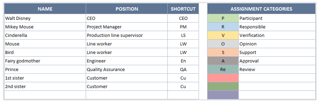
RACI Matrix

We have created a Responsibility Matrix with conditional formatting. When the user selects the assignment category for each task and each person, the template gives the colors automatically:

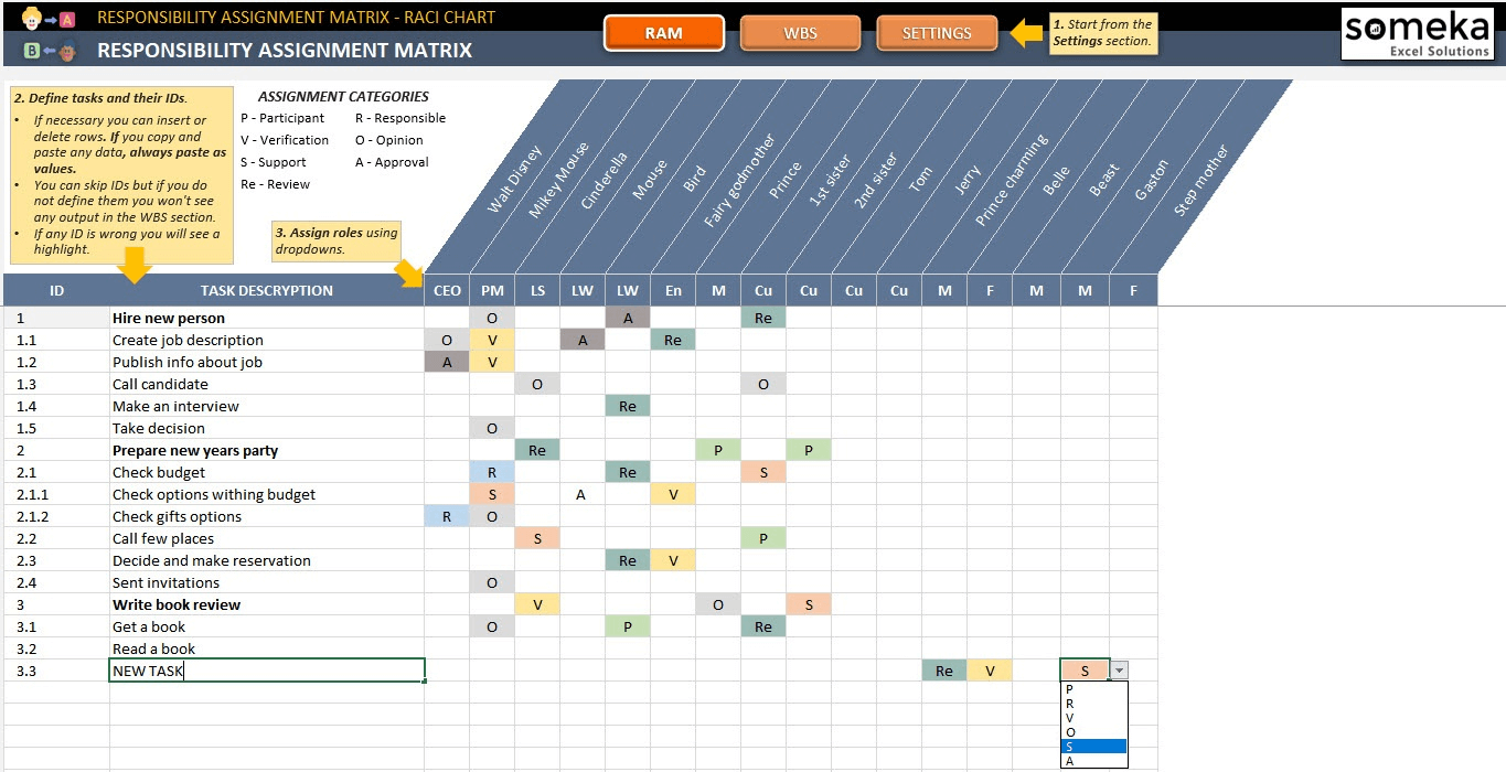
– This is the Dashboard of Someka Responsibility Matrix Template –

If you also wonder, where these colors come from, we give this as a setting to the user. So this makes the template dynamic. The user can change the category names matching the given colors:

Kanban Board View

Kanban view is one of the most unique applications of conditional formatting. First, we create the complex formulas on the backstage and then create the Kanban Board with colors:

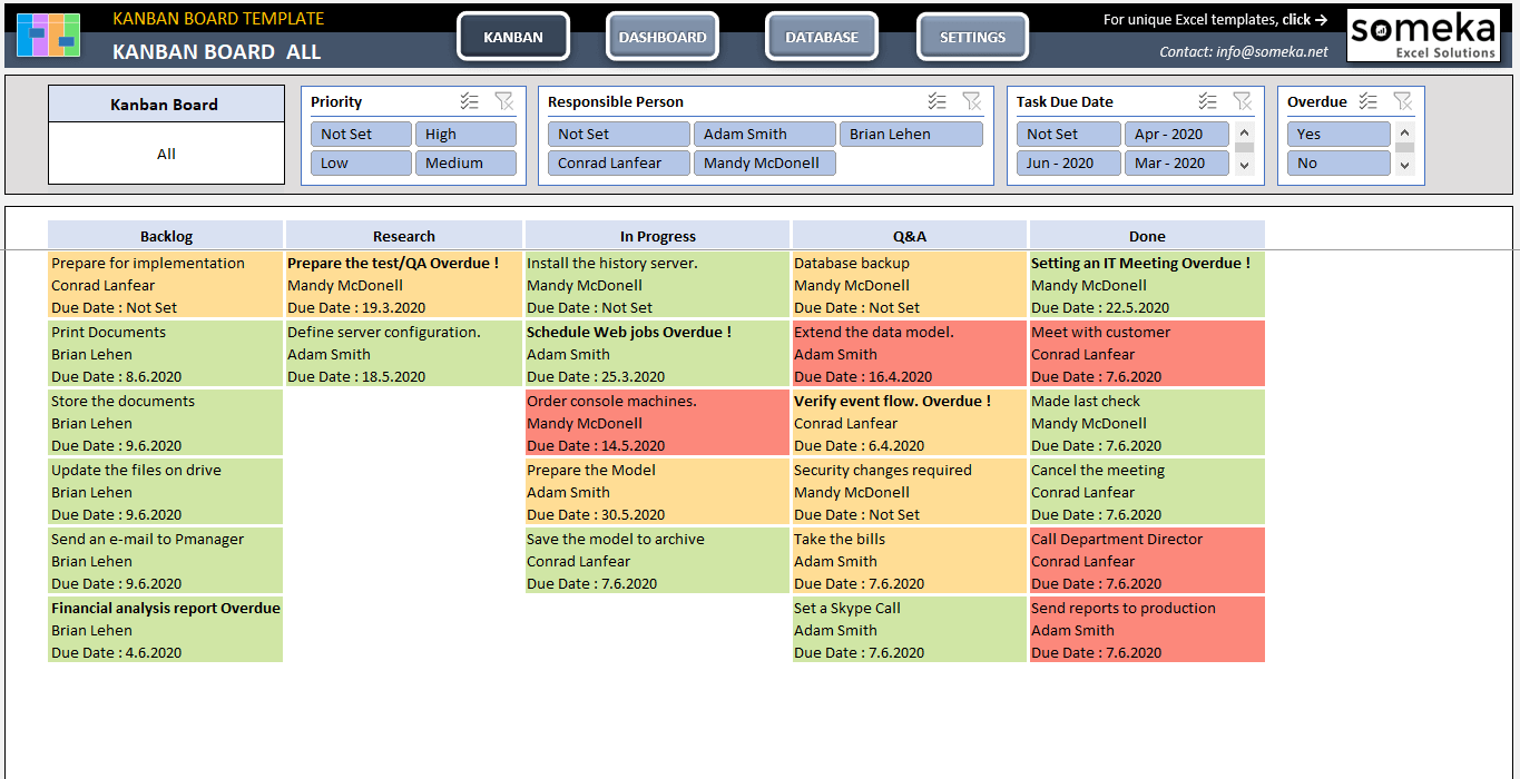
– The main section of Kanban Board Template by Someka –

In this template, all the formulas are fully dynamic, allowing for changes in any task status and priorities. For instance, if a task status is updated in one section, it reflects across the template, accompanied by changes in formatting.

The conditional formatting rules in the Headings of the Kanban view are based on the length of the cell content. For example, if a cell is not empty, it is formatted in blue.

For priority calculation, we use a table to determine the level of priority and then apply corresponding formatting to each priority level. High priorities have a red background, while the low priorities have a green background.

As you can see, conditional formatting allows for extensive customization.

KPI Dashboards with Excel Conditional Formatting

Yet another wonderful example for conditional formatting. The users of KPI dashboards usually want to see the Good and Bad results at a glance. Here you can use icons or color heat maps to underline the bad and good results.

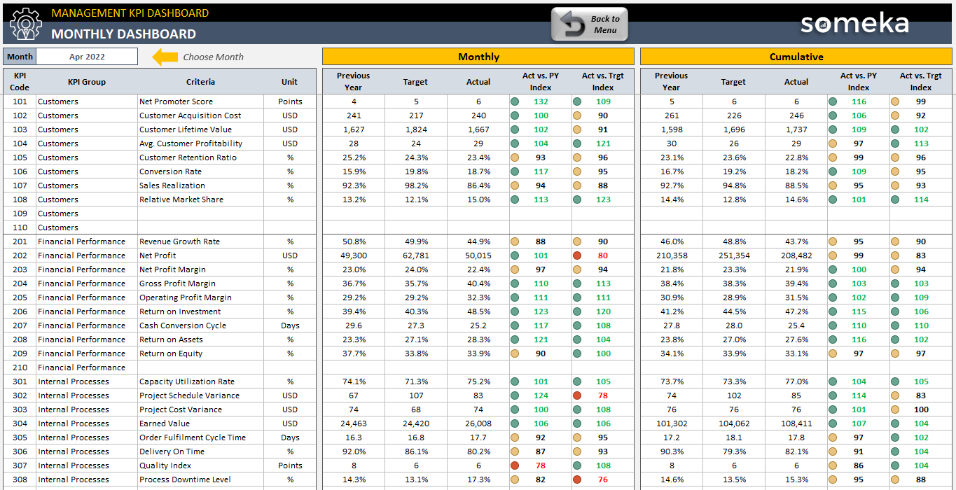
– This is the analysis section of our Management KPI Dashboard template –

First we calculate the Actual vs Previous Year and Actual vs Targets indices, then we apply conditional formatting with tiny icons. This give a clean, but powerful analysis visualization.

Roadmap

Now we’ll also give an example from our Roadmap chart.

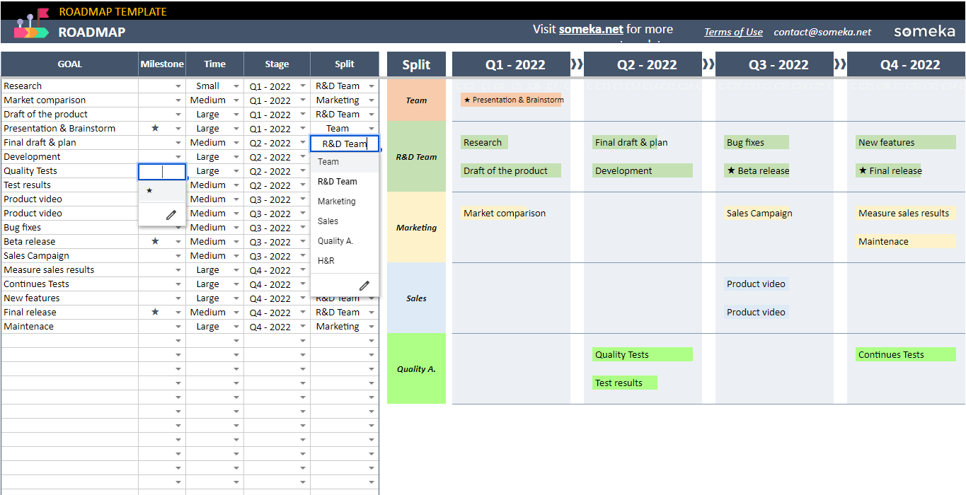
– Excel Roadmap Template from Someka portfolio –

This template mainly creates a roadmap from a list of goals. The colors are coming from the splits.  We give highlights with conditional formatting. Again the colors are dynamic and configured in the settings area.

Visible / Invisible Elements

If you want to make some elements of your file invisible unless certain conditions are met, then conditional formatting is the best way to use. In our Action Plan Excel Template, the navigation buttons for each goal only becomes visible when we write a goal.

So if the goal area is empty, the navigation button of Go to Goal is not visible to the user. This is smart, isn’t it?

Team PTO Tracking

If you want to create a PTO tracker for your team, you can make nice-looking views with Excel conditional formatting.

For example, you can create Gantt views to see the whole team at a glance:

– This is the team tracking section of Leave Tracker Template by Someka –

In the above example, you can see which employees are on vacation and with the color-reading you can understand the vacation of each one.

Another nice example here would be coloring the yearly calendar for a specific employee:

– This is the employee tracking section of Leave Management Excel Template of Someka –

Here the idea is to color the days that the selected employee is on leave. Again very dynamic layout, as the user can select any employee from the drop-down menu, and the calendar updates automatically.

We make this kind of calculations on a separate sheet and code each leave type with a single number. So, when the employee changes, the numbers update and the dashboard also changes automatically.

Employee Skills Matrix

Another very common usage of conditional formatting is competency matrix.

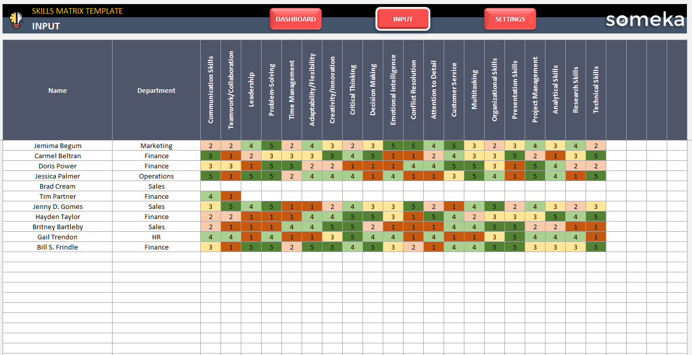
– The dashboard of Someks’s Skills Matrix Excel Template –

You can see the general heat map of your talent pool here. This is also very basic set of formatting rules. The crucial part here is to use the minimum number of rules with smart configuration in order to prevent your file slowing down.

WBS Structure

An additional noteworthy feature of conditional formatting is its ability to create simple yet effective visualizations, like a chart resembling a work breakdown structure. This is achieved entirely through conditional formatting, allowing the chart to dynamically change appearance based on various conditions.

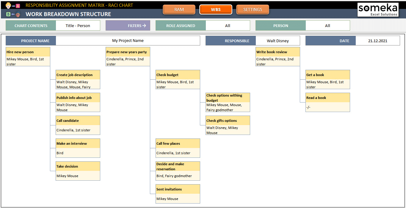
– The WBS chart area of Responsibility Matrix Excel Template –

For example, it can highlight specific roles or persons involved in a project. The versatility of these filters allows for simultaneous use or singular application, depending on the need.

A particularly interesting application we want to highlight involves dynamically adjusting borders between groups based on the number of entries within each group.

For instance, if a new task is added to a specific group, such as Q4, and labeled, say, ‘Marketing’, the formatting adjusts automatically. The borders between the groups shift down as more tasks are added, ensuring a seamless and adaptive visual representation.

Dynamic Employee Forms

Lastly, you can also create dynamic form formats with conditional formatting. This allows the user to create his/her own form template.

Below is an example of a dynamic form we’ve created for HR departments. The headings of the form is selected by the user. And all the borders and background colors are adjusted automatically according to the choice.

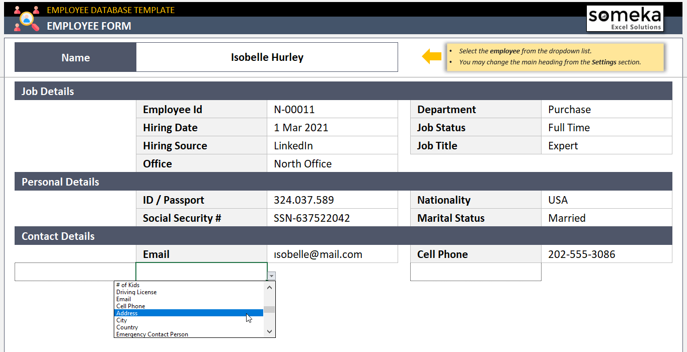
– This is the form section of Employee Database Template by Someka –

The heading options here are coming from the employee database headers. So, the HR manager can select any info header to include in the Employee Form

Conclusion

Excel conditional formatting is a powerful tool used in data visualization and analysis, enabling users to quickly identify trends, anomalies, and patterns in a dataset. This feature, widely available in spreadsheet software like Microsoft Excel and Google Sheets, allows you to apply specific formatting rules to cells based on the data they contain.

The essence of conditional formatting lies in its ability to turn raw data into visually compelling information, making it easier to comprehend and analyze. We have tried to give you some advanced tips and application examples here to get you deeper into this powerful feature.

In summary, conditional formatting is not just about making spreadsheets look more attractive. It’s a critical functionality that enhances data comprehension, aids in decision-making, and drives efficiency in data analysis.

Recommended Readings:

Excel Pivot Tables: Most Comprehensive Guide Ever with Real Pro Tips

How to Prevent and Solve Data Discrepancy Issues in Excel?

Excel Dashboard Design: How to make impressive Excel dashboards like Someka does?