How to Format Input Tables in Excel? – The Most Comprehensive Guide on Web
In this post, we’ll explain how to format your input tables in Excel? These are all standard reference tips for our developers. So, why do the input tables in Someka templates look beautiful? Here are the secrets of Excel input table formatting.

Table Of Content
1. Exporting Raw Data
2. First Quick Changes
3. Shrink-to-fit Texts
4. Columns Widths
5. Excel Date Formats
6. Excel Number Formatting
7. Alignments on the Columns
8. Separate Calculated Areas
9. Protection of the Formulas
10. Column Order
11. Summary
We’ll give tips one by one with examples and images.
1. Exporting Raw Data
Let’s start by opening a blank file. Now we’ll open a sample data file as well. You can export this sample data from an external source. It could be in Excel, CSV file, or another format.
You can use Export data options or just copy and paste your data.
We always recommend using Copy as Values while exporting data tables. You can use CTRL+Alt+V shortcut to Paste As Value.
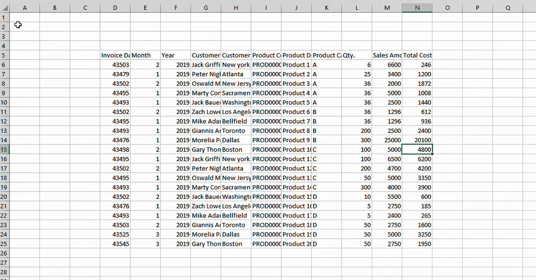
Firstly, this is how our raw data looks like. It’s a raw info columns, and we’ll make this table look beautiful and user-friendly.
2. First Quick Changes
In the first place, we’ll make some quick changes to have our raw input table look more structured.
- Select all sheets with CTRL+A
- Change the background color to light gray (hex code: #F2F2F2)
- Give borders
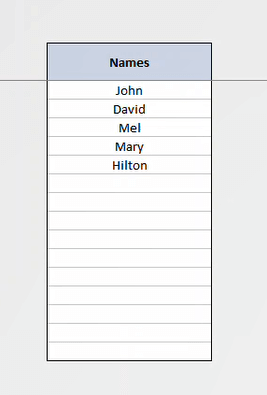
- Give the headers a color
- Make the headers bold
- Give Wrap-Text for the Headers
Now this is how our table looks:
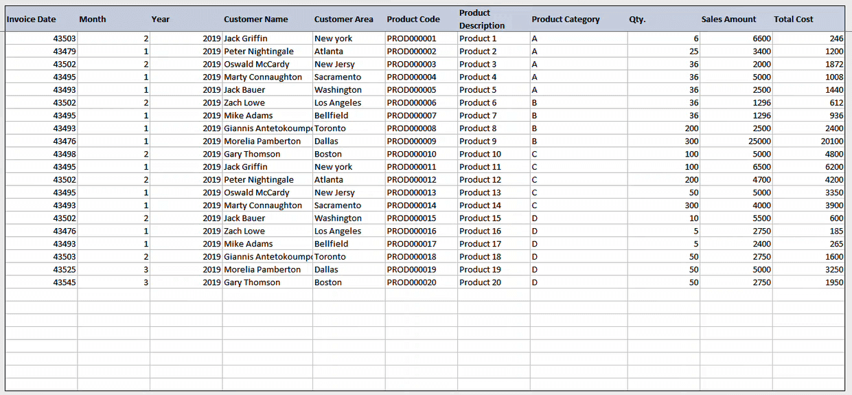
Let’s continue!
3. Shrink-to-fit Texts
Especially for long text areas, shink-to-fit is a lifesaver. You can just make your columns shrink-to-fit so that the long text does not overwrite the next cells, and also you can see the whole text.
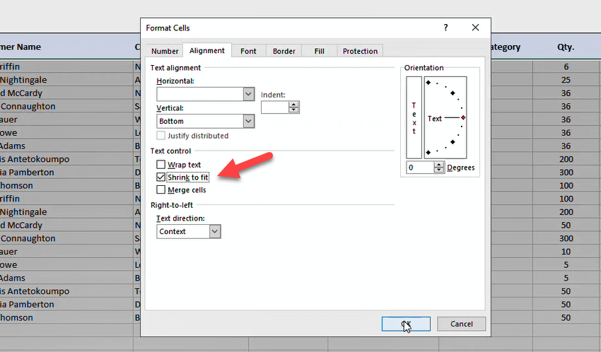
Shrink-to-fit makes the full text visible, while decreasing the font sizes in a cell. So you cannot use shrink-to-fit and wrap-text together, you should choose either of them
4. Columns Widths
You may be wondering why column width matters. Not only should it be set automatically, but it should also look good. And we pay attention to it to make sure everything looks nice. Why is the appearance of one data table superior to another? It’s because every little detail has been carefully considered.

We input our raw data into the table right away. If we use auto-fit feature, then the auto-fit will only consider the length of headers, which we do not want. So we highly recommend to fix your widths manually.
For example, you can change the column width to accommodate data that you paste from another source.
For instance, it might not fit the content properly if I just leave the column width set without manually changing it. In the event that a header requires only one line and changes, the automatic adjustment may not function as intended. For this reason, we like to set it to guarantee consistency whether the content is lengthy or not. Additionally, we want to be in charge of the row heights.
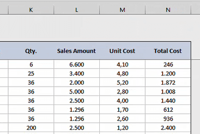
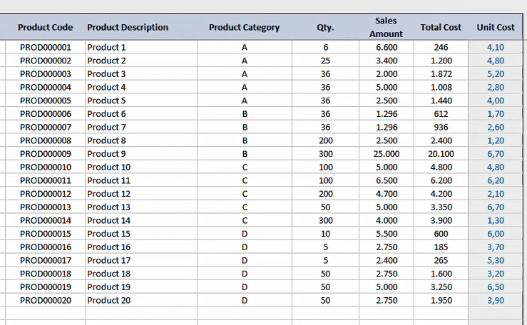
Another cool tip about column widths is using the same Width for similar input columns. For example for Sales Amount, Unit Cost and Total Cost columns will have similar data inputs. So we can use the same column width for all these columns.
5. Excel Date Formats
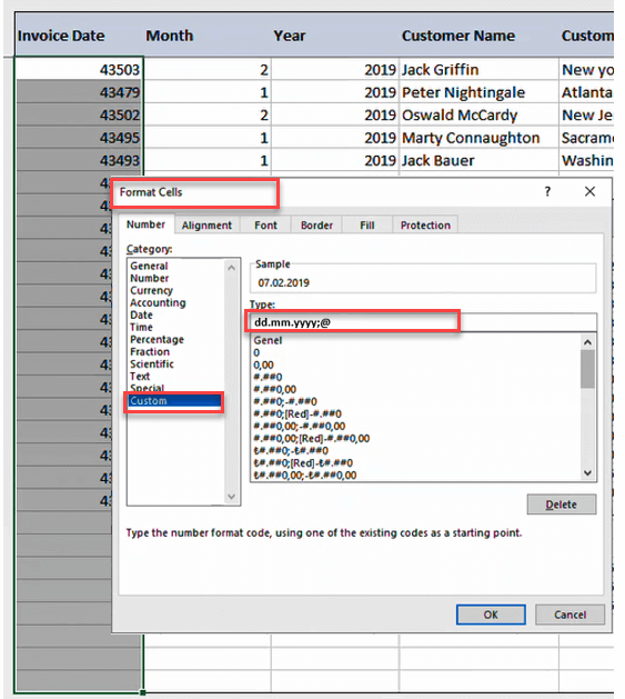
Now we’ll format the date columns.
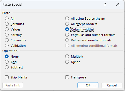
After opening the Format Cells box with CRTL+1, go to Number > Custom and type your custom formatting. You can also choose one of the given formats under the Date section.
6. Excel Number Formatting
Then, we’ll format the numbers. Again open the Format Cell box and go to Number to configure your best suitable number format.
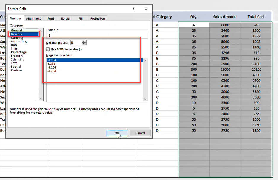
As a general rule, decimals must be displayed. However, very large figures should not contain decimals. For example, you don’t always need to use decimals to be extremely precise when dealing with big quantities such as $25,000. Because $25,000 is not meaningfully different from $25,000 and 16 cents.
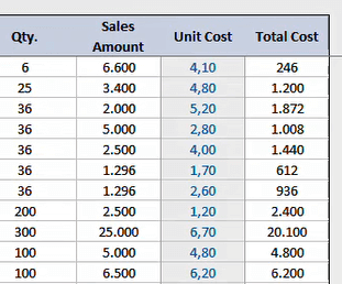
This is an important tip. We can omit the decimal places for large numbers. However, it’s crucial to include them for smaller amounts, like unit cost.
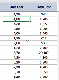
For example, you can easily ignore the decimals for total costs, where the amounts may surpass hundreds, or even thousands. On the other hand, you should have two decimals for the unit cost. Because rounding these unit cost numbers will change the story.
7. Alignments on the Columns
Firstly, you can align your columns to left or make them centered. But which one to choose? Here the tip:
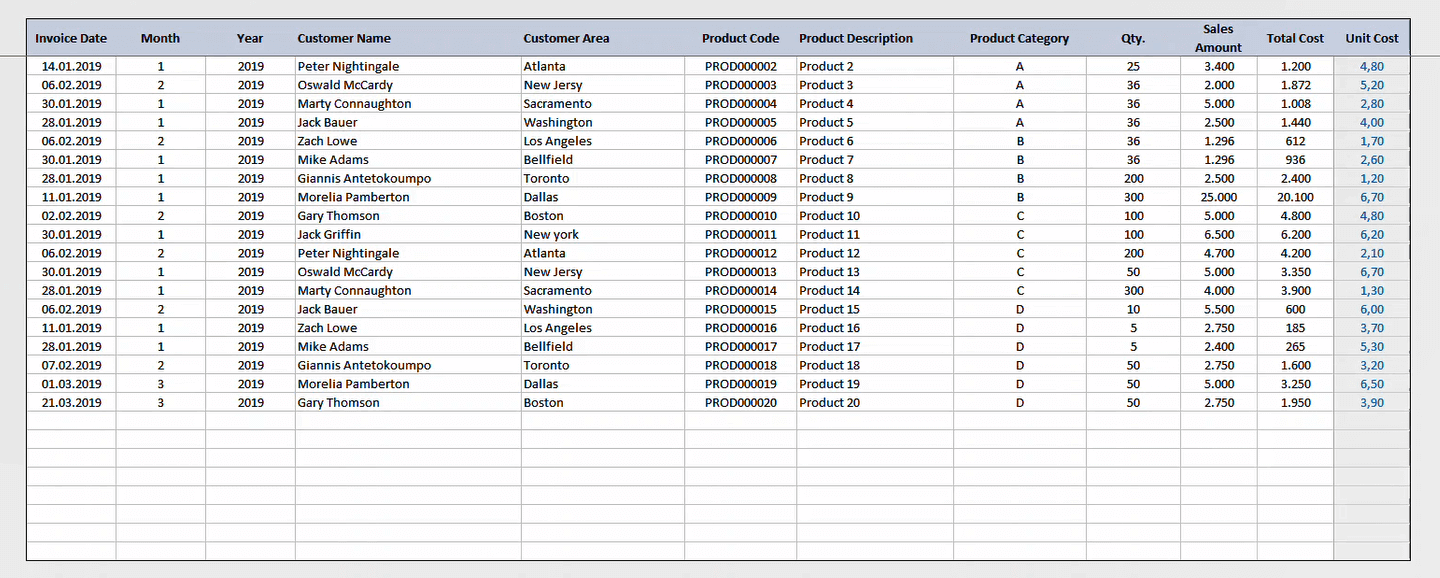
Text should always be aligned to the left when working with it, especially long texts like addresses, business names, or customer names. Centered texts look odd and it is not typical to the human eye, particularly when it comes to items with flexible lengths like names.

Centering, however, can look good for items like product codes, which have a more uniform length. As a general rule, centering can be effective if the content does not vary significantly in length. It is preferable to align longer texts to the left side.
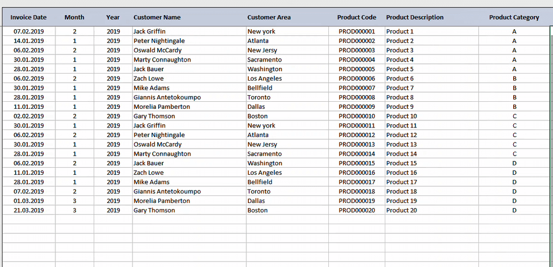
For instance, the length of product descriptions must be flexible. It won’t be enough if we leave a very short column width here. Therefore, we ought to make more room for in-depth descriptions.
The product category may have an identical width, so we can center this column.
8. Separate Calculated Areas
You’ll have two types of areas in data input tables:
- Data input areas, where the user will paste or write data.
- Calculated areas, where you have your Excel formulas
In Someka templates, all areas in our table or input layout are typically colored in grey, with the exception of the areas where users or customers will enter data, which is left white.
For clarity’s sake, we may also demarcate these areas with borders. You can also change the Font colors to blue or something else to make it clear that these areas are different from the input areas.
Let us show you an example of this method’s implementations in our portfolio:
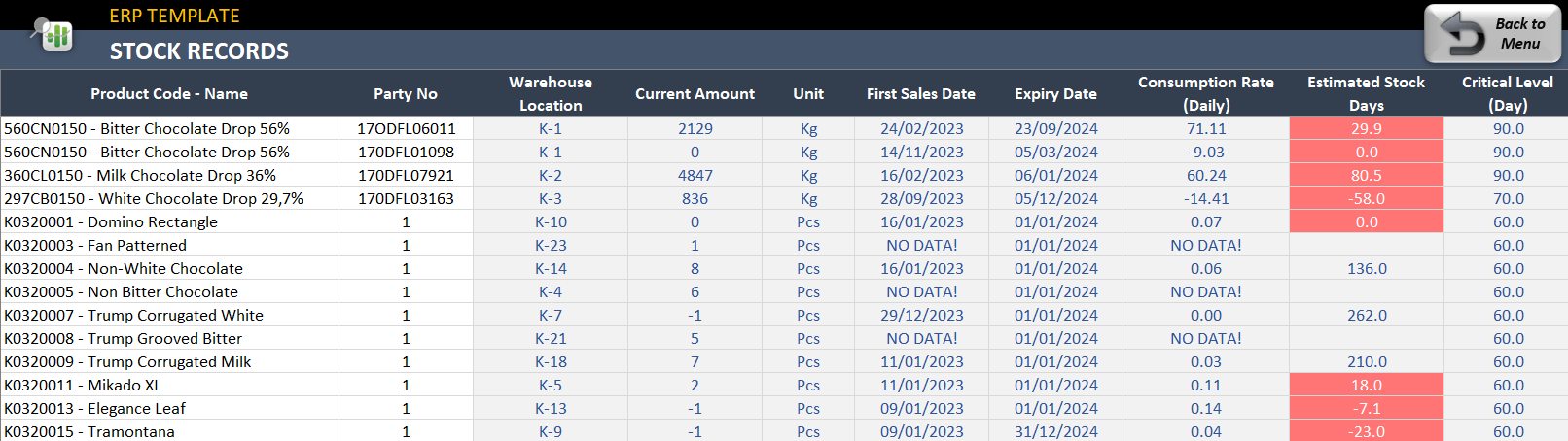
This is a screenshot from our ERP Excel Template. As you see, most of the columns are calculated areas. The user will only input Product Code and Party No here. All the other areas are calculated automatically.
Sometimes, we don’t color everything blue if there are too much of calculated areas. The goal is to make the editable sections stand out while making the non-editable portions obvious.
9. Protection of the Formulas
You can protect your sheets to prevent any user fault on the formula areas. Here you have to do two things:
- Unlock the data input area
- Protect your sheet with or without password
If you do not unlock the white data input areas before protecting your sheet, then the user will not be able to input or paste data in those cells. So exclude your data input areas from the protected sections.
How to unlock input areas in a protected sheet?
Open Format Cell dialog box with CTRL+1, go to Protection and uncheck the Locked box.

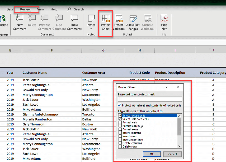
Now we’ll protect our sheet.
How to protect your Excel sheet?
On the top menu, go to Review > Protect Sheet. You can also define a password here if you want.
10. Column Order
But there might be a problem with our data still. Suppose someone wishes to copy data from another file into our table. They are unable to just copy and paste their data into a locked portion of the table. They would have to tediously copy and paste each piece one at a time.
Thus, it’s important that our tables be easy to use. In order to avoid interfering with the user input area, it is preferable to position formulas toward the right side of the table.
Now our formulated column is carried to the right-most side of our data input table. This is the last tip of our Excel input table formatting post.
For instance, list the category first, then the subcategory, and finally the particular item details. This order makes more sense and is simpler to comprehend. However, if some information is less relevant, it might be better positioned toward the end of the table depending on the context.
Now, out Excel input table looks nice and clean!
11. Summary on Excel Data Input Formatting
This is how we can quickly format our data input table with expert tips. This will give our Excel tables a much more beautiful look.
As a key takeaway, our usual procedure is to color the header, clear the content, and then make necessary width and alignment adjustments. Just have simple and clean looks in your tables.
This structure is set for ordinary input data tables, but keep in mind that Excel offers additional table formatting options. We’ll explain the details of Excel Tables with advantages and advantages in a separate post. Stay tuned for more tips!
Recommended Readings:
Excel Dashboard Design: How to make impressive Excel dashboards like Someka does?
Related Posts