Excel Pivot Tables: Most Comprehensive Guide Ever with Real Pro Tips

In this article, we’ll try to share our deep expertise with Excel Pivot Tables. You will find some very rare tips here, that you cannot see in ordinary pivot table tutorials or posts.

This article is created from the internal training tutorials prepared for Someka interns. So you’ll find to-the-point expert tricks here!

Let’s begin!

Table Of Content

1. What’s the logic behind Excel Pivot Tables?
2. First 3 Things To Change
3. Pivot Table Quick Layout Design Options
4. Naming Pivot Tables
5. Pivot Table Advanced Design
6. Date and Number Formatting in Pivot Tables
7. Bonus Tip: Finding Data Discrepancies With Pivot Tables
8. Final Words

1. What’s the logic behind Excel Pivot Tables?

Firstly, we’re going to talk about the basic logic behind pivot tables.

What an Excel pivot table actually does?  This is one of our interview questions for our Excel developer candidates:

If you were to perform the same operations as pivots using formulas, which formulas would you use?

The answer is very easy. In addition to other features, pivot tables essentially make groups of data according to selected criteria and then counts, sums, get averages of that groups.

Essentially, what Pivot Tables do is this: They perform certain operations on data in a specific way, like counting or performing other operations rapidly.

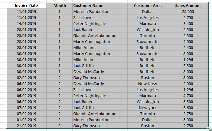
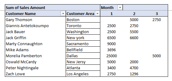
Let’s give an example. Below is our raw data source:

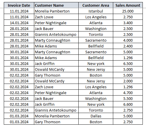
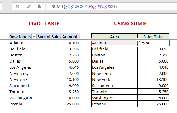
Now we want to calculate the total sales amount for each area. We have two options. We can use Pivot tables, or we can use SUMIF function.

The greatest beauty of a Pivot Table is its ease of manipulation and speed. Its working mechanism is different from formulas, storing data in a unique cache within the Excel file.

We’ll cover some very basic things about creating a Pivot Table. Let’s start with a blank Excel file and source data.

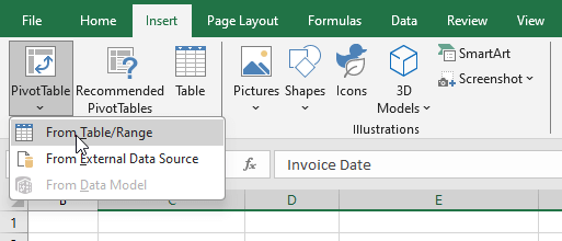
It’s very easy to add a pivot table: Select your source data and go to Insert > Pivot Table > From Table/range.

But where to add your pivot table?

It automatically suggests you ‘New Worksheet’. But it doesn’t have to be this way. We can also select the same sheet with the source data. For example, we can select the data and immediately sort it out on the same tab, without creating a new sheet.

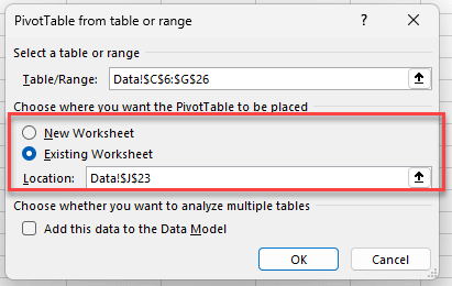
Note: There’s also an ‘Add this data to the Data Model’ option. We’ll cover this later.

If you’re linkink more than two tables, then you should master power pivot for excel, which provides easy way to create pivot tables and charts from complex data models.

2. First 3 Things To Change

The first thing we recommend doing right after creating a Pivot Table is going to options and:

1. Remove auto-fit column widths on update
2. Check box for Error Values show blank
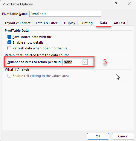
3. Go To Data tab and Make Number of Items to Retain per Field as None

Let me explain what these changes mean:

Auto-fit

When you leave this auto-fit option checked, then it automatically adjusts the width of columns. Auto-fit can be useful depending on the situation, but we usually manage our Pivot Tables manually, so we don’t need it. It’s more for layman users who might accidentally mess up the layout.

So the default setting is auto-fit in Excel, because it’s better to have an ugly layout than an invisible one. But you’ll not need that thing when you become and powerful Excel pivot table user.

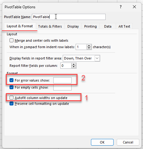
Show Blanks for Error Values

It’s for error conditions. Let’s say we’re calculating something and there’s a division by zero. Normally, an error would show up, but we don’t want that in our Pivot Table.

Instead of showing an error, we want it to show a blank. In our experience, this is usually better, but please remember there might be situations where you want to see the errors.

Retain deleted items?

As mentioned above, the Excel Pivot Tables work with a caching logic. That’s why they are fast.

But when caching, Pivot Tables ask you, “Do you want to retain items deleted from the data source?”

Sometimes, there could be logical reasons to keep them. But generally, we don’t want to keep them as it causes confusion. Imagine you add a dummy data or a wrong data, and then delete it. But if you leave this fetaure open, it will retain all deleted items even if they do not exist in your source data anymore.

In summary, when creating a Pivot Table, the first three things to do are: Go to options and 1. Remove auto-fit, 2. Show blank for error, and 3. Set the retain value to No Data. These steps should become automatic.

3. Pivot Table Quick Layout Design Options

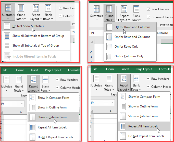
We’ll not give you some tips about the Pivot Table quick design. For a clean view at the first glance, we make these four changes:

1. Do not show subtotals
2. Grand Totals off for Rows and Columns
3. Report Layout show in Tabular Form
4. Report Layout Repeat All Item Labels

Here’s the summary of these four changes:

Tabular Form design is a preference, but it helps in clear data analysis. Because, it looks nice and maintains clarity.

Additionally, you can also remove the plus/minus buttons for expanding and collapsing. We usually remove those for a cleaner look.

Other layout forms may look more stylish, but for data analysis reasons, these options make it easier to copy your pivot data and make a separate analysis or get the pivot table of your pivot table.

But maybe after all your analysis is done, you can prefer other cool layout designs for your final report or dashboard.

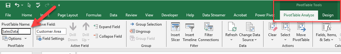
4. Naming Pivot Tables

Also, always give your Excel Pivot Tables descriptive names. This helps in identifying them, especially in complex scenarios. It’s a good practice, even if you don’t always use it.

Especially while adding slicers or charts, this name will help you a lot.

How to name a pivot table?

Under the Pivot Table Tools > PivotTable Analyze, you can replace the default name with a more descriptive one.

5. Excel Pivot Table Advanced Design

Now, let’s talk about Pivot Table design, a feature many people don’t often explore. You can make various changes from the design tab. For instance, if you don’t like the bold row headers, you can choose to remove that formatting to make the table look cleaner.

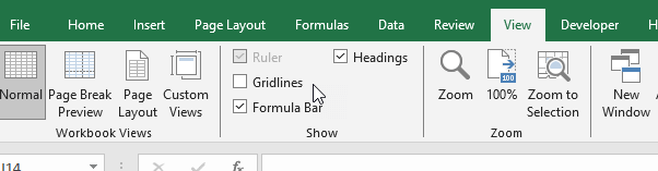
Firstly, if you’re adding your pivot table to a separate sheet, feel free to remove gridlines for a more beautiful-looking layout.

Secondly, you can modify the column widths according to your data. Additionally, you can decide on the alignment of your data. If the length of data varies a lot, we recommend to align them to the left. If the input data is mostly in the similar length, you can use Center option.

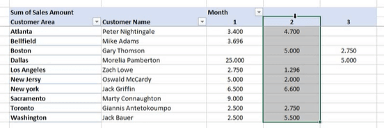
While designing your pivot tables, always use the little arrows to select the pivot columns. Otherwise, when you add new data and refresh your pivot table, it will not keep your design!

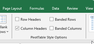
Then, you can select your Style Options with the related checkboxes. You can, for example, turn of Raw Headers if you do not need them.

It’s important to note the difference in selecting ranges when applying changes. If you select the entire Pivot Table and apply a format, it will apply to the entire table. But if you select just a column or a specific area, the formatting will apply only there. This distinction is crucial for understanding how your changes will affect the table.

Custom Pivot Table Design

Many people don’t know that you can create your custom Pivot Table design.

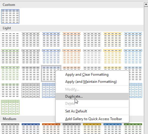
To do this, you first duplicate an existing design and then modify it to your preference. To create a duplicate, right click on any default design under the PivotTable Styles, and click on Duplicate.

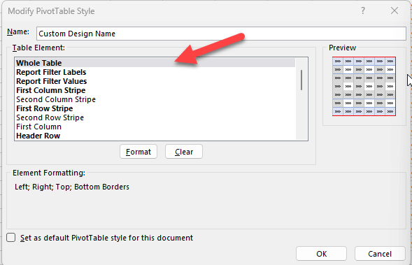
Then give a custom name to your design.

For example, you can change the header row text to be non-bold or adjust the formatting of the first row stripe. This is how you can create a unique design that suits your needs.

In order to modify your custom design, click on the Design element you want to change, and then click on Format.

Let’s explore more in-depth Excel Pivot Tables. Say you want to add a border around the entire table. You can choose a color and apply it, which is a rare but useful customization. Another tip is to remove gridlines for a cleaner appearance. You might also want to change the color of the row stripes. When modifying, you can explore different options to find what works best for you.

Remember, default designs in Pivot Tables come with certain pre-set styles, like bold headers. When creating your design, you’re free to change these elements. This customization can be very useful, especially if you need a specific look for your Pivot Table, like in a corporate template.

How to add red outside borders to our pivot table?

First we’ll select the whole table as our table element:

Then we’ll click on Format, and make the desired change on the Format dialog box:

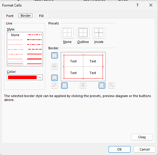
Now our table has a red border.

Below is a good example from custom pivot tables:

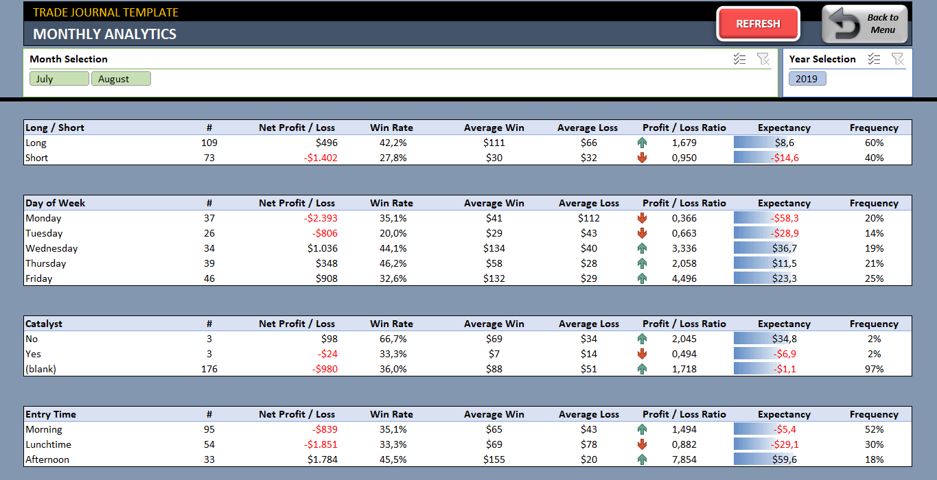
– This image is from Someka’s Trade Journal Template which has a professional looking with custom pivot table designs –

A unique trick to know is how to apply a border. If you apply a border directly to the Pivot Table and then refresh it, the formatting might get messed up.

Instead, apply the border to the cells around the Pivot Table. This way, the border remains intact even after refreshing.

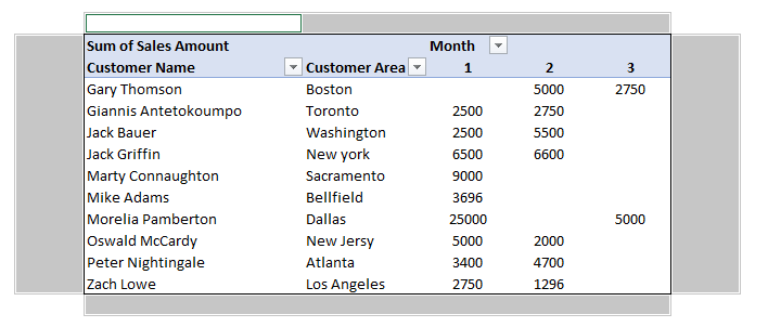
However, be aware of a downside to this method. If new data is added to the Pivot Table, the border won’t automatically adjust to include it. For a more dynamic and adaptable design, it’s better to create your custom design in the Pivot Table’s design settings. This way, the design will automatically adjust to changes in the data.

Remember, your design choices should facilitate easy reading and interpretation of the data. For example, when calculating averages, ensure that the formatting will apply to future data entries as well. This keeps the table dynamic and responsive to new data.

In conclusion, the key is to balance functionality with aesthetics, keeping in mind how the data will be used and interpreted. That way, you create a Pivot Table that’s not only informative but also user-friendly.

6. Date and Number Formatting in Excel Pivot Tables

A common problem with Pivot Tables is formatting the data in the rows section, particularly when trying to change the number format.

You might find that changing the number format in the usual way doesn’t always reflect in the Pivot Table, even though it seems to change in the cell itself. This is because Pivot Tables handle data differently, and their design ensures certain limitations.

So you should always change your date and number formatting under the Value Field Settings of your Pivot Table.

But what if you cannot see these settings?

Here’s a pro tip for you:

To change the format, you need to ensure that the entire column in the source data is formatted as a date, with no blank spaces or text. If you try to change the format while there are blank spaces or non-date elements in the column, it won’t work. This might require you to clean up your data, removing any blanks or non-date elements from your source data.

Another important point is that if you have slicers connected to your Pivot Table, they can prevent you from updating the data source. You need to remove these connections first before making changes to the source data.

So if the date formatting is not active, there might be two reasons behind that:

1. You may have blank rows on your source data
2. You might have slicer connections related to that pivot table

So in order to change the date or number formatting, first remove the slicer connections and make sure that you do not have blank rows on your source data.

Dynamic Sources in Pivot Table

Here’s a useful tip:

Create a dynamic range for your source data. This way, your Pivot Table will automatically adjust as your data grows, without including unwanted blank spaces. You can create a dynamic range using an OFFSET formula on the Name Manager that adjusts the height and width of your range based on your actual data size.

Firstly calculate the height of your dynamic range with MAX formula, then go to Name Manager and use OFFSET formula and reference to the MAX formula cell as the height of your Offset data range.

Only for Pros:

Why you can not change formatting on the blank source data?

Here’s the answer. If you unzip your Excel file (yes, you can unzip your Excel files!), you will see that all the elements are actually XLM documents in that zip folder.

Pivot tables are also recorded XLM files, and if you have blank spaces in your raw data, then it sees your source data as Text format. But, in order to keep your pivot column in date formatting, all your data should be in date format. That’s why you cannot change the formatting if you have blank rows inside your data.

The key takeaways of this section:

• Understanding the limitations and restrictions caused by slicers in Pivot Tables
• The importance of not leaving blank spaces in your source data for effective formatting within Pivot Tables
• Creating a dynamic source data range for your Pivot Tables
• Understanding how Pivot Tables process and store data, affecting how you can format it

7. Bonus Tip: Finding Data Discrepancies with Excel Pivot Tables

We’ll now demonstrate a highly useful but simple operation with Pivot Tables.

Let’s assume you have a set of data and you want to ensure that certain codes match up exactly without any discrepancies.

For example, if you have a code 162 corresponding to S102 in one place, you want to make sure it doesn’t accidentally correspond to S110 in another. This is essentially ensuring a one-to-one relationship.

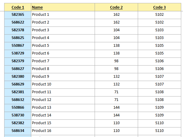
To illustrate, suppose you have product codes and corresponding values. You want to make sure that each product code matches with one and only one value.

For instance, code 162 should only match with S102, and not be found matching with any other value in the dataset. This verification is crucial, particularly in cases where you’re matching product codes with something else and you need to be certain that each code is used uniquely.

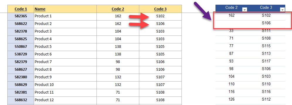
To check this in a Pivot Table, you first arrange the codes side by side. By setting the Pivot Table in tabular form and turning off the grand totals and subtotals, you can easily see if there’s a one-to-one match.

If a code corresponds to multiple values (or vice versa), it would be evident.

A Case Study:

For instance, if code 162 is set to match with S102, but you also find it matching with S106 elsewhere, it would be clear that there’s not a one-to-one relationship.

You can check this by observing the layout of the Pivot Table – if there are multiple entries for the same code, it indicates multiple matches.

However, to be completely sure of a one-to-one relationship, you need to check this from both directions. This means you arrange your data in one order (e.g. code 2 then code 3) and then in the reverse order (code 3 then code 2). If in both arrangements, each code and each value appears only once, you can be confident that there’s a one-to-one relationship.

This method, while a bit complex to understand at first, is an effective way to ensure the accuracy of data relationships in your dataset. It’s particularly useful in scenarios where maintaining a strict one-to-one match between elements is crucial.

8. Final Words

In this article, we have tried to give you quick and pro tips about Excel pivot tables. No doubt, pivot tables are one of the most unique features of Microsoft Excel. As data analysis tools, pivot table should be your first address in the road to becoming a powerful Excel user.

Recommended Readings:

Excel Dashboard Design: How to make impressive Excel dashboards like Someka does?

How to make your Excel files look MUCH better?

Career Guide: Data Analyst