How to Highlight Duplicates in Google Sheets

In this blog, we will show you how to highlight duplicates in google sheets. It will make your spreadsheet more advance and easy to follow. You can use the below formula to highlight duplicates in google sheets. The formulas that we will give you about google sheets conditional formatting duplicates and after this blog you will be able to highlight duplicate cells easily. Also, you can find the answer for how do I filter duplicates in Google Sheets. Moreover, there are answers for the people who look as ” how do I find duplicates in google sheets ”

How to Highlight Duplicates in Google Sheets

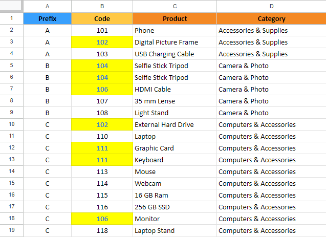
Firstly, Let’s check the example below to highlight duplicates:

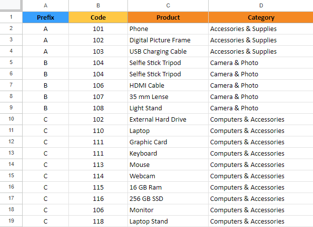
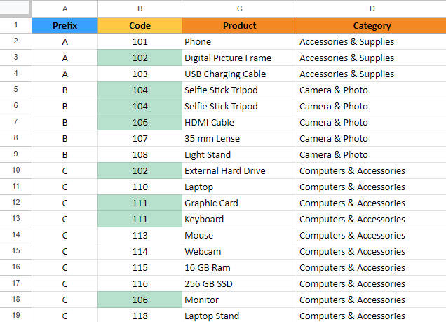
Secondly, we can highlight duplicate cells in the code column.

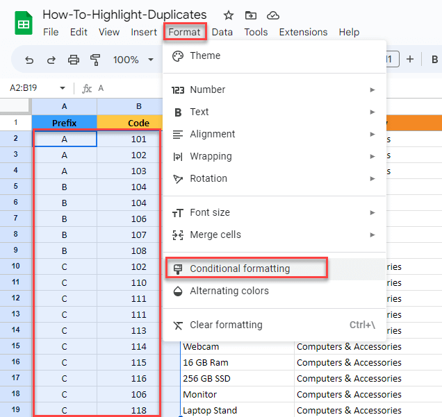
1- Select the Code

Moreover, select the code column (B2:B19) and go to Format ->Conditional Formatting

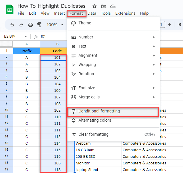
Now you will see Conditional Format Rules on the right side of the screen. Be sure that the “apply to range” section is correct.

2- Go to Format rules

Go to Format rules and select “Custom Formula is”.

3- Use the Formula

Use the below formula to highlight duplicates in google sheets

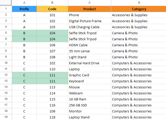
Formatting style can be changed in the Formatting Style section in Conditional Formatting Rules.

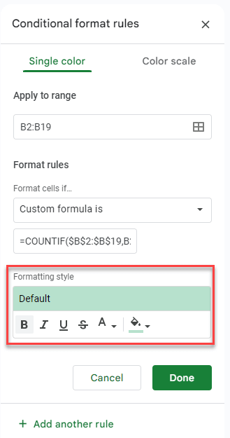
For example, you can see the changed formatting style with bold, blue font color and yellow fill color.

Google Sheets highlight duplicates in two columns

If we want to highlight duplicates in multiple columns, we can use the method below.

Then ,select the range to find duplicates and go to Formatting -> Conditional Formatting

As well as, we use the ARRAYFORMULA in the COUNTIF formula.

As a matter of fact, you can extend the number of columns using the “&” expression to find duplicates. The most important part is the number of rows for each column should be the same.

How do I filter duplicates in Google Sheets?

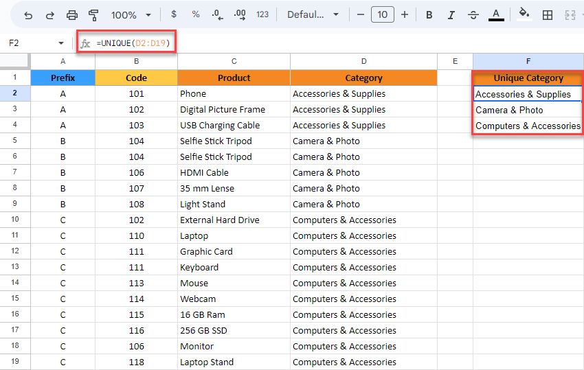
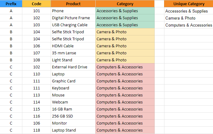
Using the “Unique” function we can filter duplicates in Google Sheets. Let’s filter the category column by removing duplicates using the formula below:

Furthermore, let’s highlight duplicates in Google Sheets in the same category with the same color for each part.

Then, we will select the Category column and again go to Formatting -> Conditional formatting select “custom formula is” in the “Format cells if…” section.

Likewise, using the formula below we can differentiate each category differently.

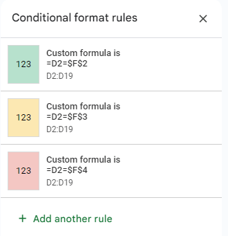
Lastly, we can easily highlight the same category with the same color.

If you like our blog ,you can check for more google sheets tips here!

Also, you can watch our Google Sheets tips videos here!