How-To-Highlight-Duplicates-In-Excel-Someka-Blog-Featured-Image

How to Highlight Duplicates in Excel? Find and Define Duplicate Values

Excel Tips
Updated on May 23, 2024

You’re working on a big data table and want to find duplicates in a row or column? So, here’s a complete guide on how to highlight duplicates in Excel with different methods and scenarios.

Table Of Content

1. How to Highlight Duplicates in Excel?
2. What is the Shortcut Key for Highlighting Duplicate Cells in Excel?
3. How Do You Select All Duplicates in Excel?
4. How to find duplicate values with formula?
5. How to Highlight Duplicates Except for the 1st Occurrence?
6. How to Show Xth and Subsequent Duplicates?
7. How Do I Show Only Duplicates in Excel?
8. How to Filter Duplicates in Excel?
9. How to Highlight Entire Row According to Duplicate Values?
10. How to Highlight Consecutive Duplicates in Excel?
11. How to Highlight Duplicates in Multiple Columns with an Excel Formula?
12. Conclusion

1. How to Highlight Duplicates in Excel?

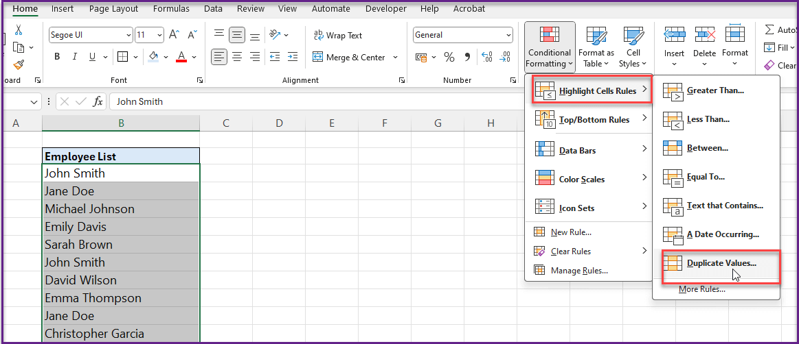
The easiest way to non-unique values is the built-in conditional formatting feature.

First, select the range, row or column you want to check for the duplicates
Then, go to conditional formatting from the Home tab
Choose Highlight Cell Rules from the drop-down menu
Then, select Duplicate Values
Lastly, select your formatting style
And click OK

Thus, the below is a simple example to highlight duplicate names in an employee list:

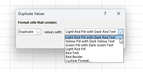
Once you open Duplicate Value wizard, you’ll define your formatting style for the duplicate values.

So, you can either select a built-in style from the dropdown menu, or you can create a custom formatting.

Actually, this method will highlight all duplicate values within the selected range, making it easy to spot them.

2. What is the Shortcut Key for Highlighting Duplicate Cells in Excel?

Microsoft Excel does not have a direct shortcut key for highlighting duplicates. But you can use a combination of keyboard shortcuts to achieve the same result quickly, which is ALT+H+L+H+D.

After selecting your range manually or with CTRL+A shortcut:

First, Press Alt + H to go to the Home tab.
Then, Press L to open the Conditional Formatting menu
Then, Press H to choose Highlight Cells Rules
Lastly, Press D to select Duplicate Values

Excel will help you with references to find your right way to the duplicate values feature. So, these steps will bring you to the Duplicate Values window, where you can customize the formatting and apply it without using your mouse.

Furthermore, you can use the same dynamic shortcut keys for other excel functions, including the remove duplicates.

3. How Do You Select All Duplicates in Excel?

To select all duplicates in Excel, you can use the filtering feature along with conditional formatting. Here’s how:

After highlighting duplicates in your list, go to Data and add Filter.

Then, filter your data according to the formatting settings.

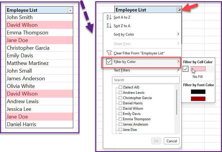
So, this method will filter the data to show only the duplicates, which you can then select and manage as needed.

4. How to find duplicate values with formula?

The built-in find duplicates feature is a handy tool, but this will not be enough forever. Especially, when you want to build more dynamic checking for the duplicate values you’ll need a more complex formula.

So, we’ll again use conditional formatting, but this time we will add some custom formulas. Our main helper will be COUNTIF() function here.

=COUNTIF( range ; first cell ) > 1

With the above rule, we’ll count if the cell is repeated in the dynamic range.

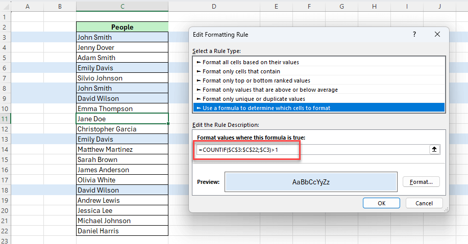
For example, we have a list with ID numbers and names. We want to highlight duplicates in Excel ID column:

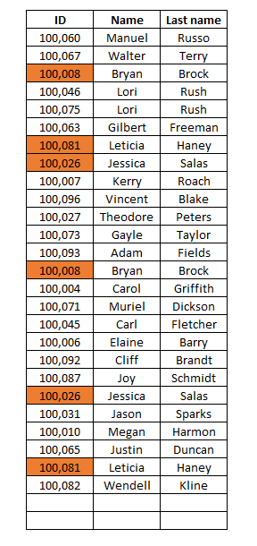
Firstly, select your formatting range and go to Home > Conditional Formatting > New Rule
Then, select Use a Formula to determine which cells to format as the rule type
Lastly, we’ll write the formula

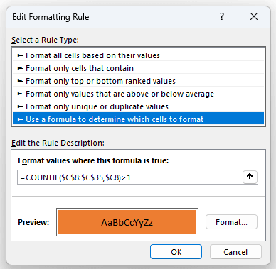
In this example, the C8 is the top cell, with C35 being the last cell of our range. The most tricky part here is about using the $ signs to set up absolute, relative and mixed references. We’ll fix our starting end end point of our range, with using a relative reference for the criteria cell. If the count number is greater than 1, this will format the duplicates according to our style preferences.

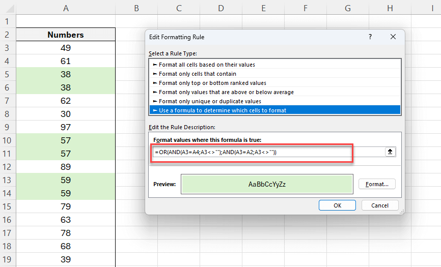
5. How to Highlight Duplicates Except for the 1st Occurrence?

Highlighting duplicates except for the first occurrence can be achieved using a formula in conditional formatting. So, we’ll only update our COUNTIF formula here to highlight duplicates in Excel, excluding the first occurence.

Select the range of cells you want to check.
Go to Home > Conditional Formatting New Rule
Choose Use a formula to determine which cells to format
Enter the following formula:

=COUNTIF( $A$1:$A1 , A1 ) >1

Now, we have created a dynamic range for our checking list. It will check the range always starting from the first cell, but ending with the related cell.

Again, the important issue here is how we use the $ signs.

This formula checks if the count of the value is greater than one up to the current cell, effectively highlighting all but the first occurrence of each duplicate.

6. How to Show Xth and Subsequent Duplicates?

To highlight the Xth and subsequent duplicates, you need a slightly modified formula for your conditional formatting rule:

Go to Conditional Formatting > New Rule after selecting your range, and select Use a formula to determine which cells to format as your rule type.

Now, to highlight duplicates in Excel with a xth condition, our formula will be:

= COUNTIF ( $A$1:$A1 , A1 )>=X

So, you can replace X with the number of the occurrence you want to start highlighting from (e.g., 2 for the second and subsequent duplicates).

Lastly, configure your the desired formatting and click OK.

For example, on the below scenario, we have highlighted 3rd and onwards duplicates. That’s why the first two of the duplicate value is not highlighted.

7. How Do I Show Only Duplicates in Excel?

To display only duplicates, use the advanced filter feature:

First, go to Data > Advanced and on the Advanced Filter wizard define your List range and Copy to range. Then, check the box for unique records only.

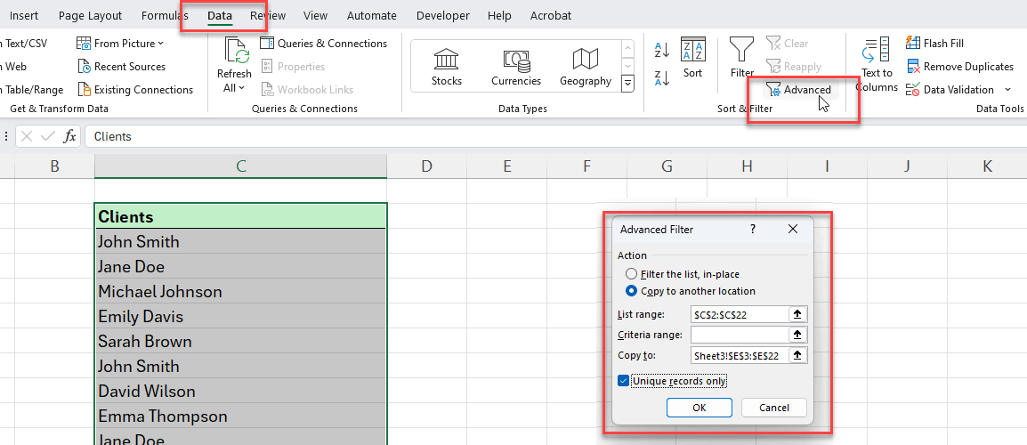
You can apply this filter to either on the same list or copy it to another location.

So, this will filter the list to show only unique records.

8. How to Filter Duplicates in Excel?

Firstly, To filter your duplicates, you can add conditional formatting and then filter them according to the colors.

Alternatively, you can use a helper column to find duplicates and then use this column as filter basis.

Let’s go with this second method which is more flexible:

First, we add a helper column
We build a IF and COUNTIF formula saying that if the count of the adjacent cell is more than 1 write duplicate, otherwise write unique

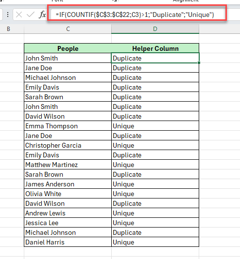
Then we’ll easily go to Data > Filter to add autofilter to filter this table:

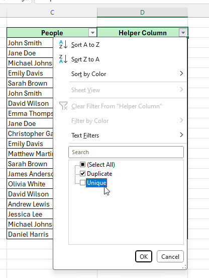
Now you can easily filter your duplicate or unique values to work more efficiently.

9. How to Highlight Entire Row According to Duplicate Values?

To highlight entire rows based on duplicate values in a specific column, we’ll again use the conditional formatting custom rules feature.

Select the entire rows of the data set
Go to Home > Conditional Formatting New Rule
Choose Use a formula to determine which cells to format
Add the below formula

=COUNTIF ( $A$1:$A$100 , $A1 )>1

This will highlight all the rows that includes duplicate values in a specific column.

10. How to Highlight Consecutive Duplicates in Excel?

Highlighting consecutive duplicates requires a custom formula:

Select the range to format
Go to Home > Conditional Formatting New Rule
Choose Use a formula to determine which cells to format

Now, we will add the below formula to the custom formula area:

=OR( AND(A3=A4,A3<>””) ; AND(A3=A2,A3<>””) )

Lastly, we will select our formatting style and click OK.

Then, this formula checks if the current cell is equal to the next cell or previous cell, highlighting consecutive duplicates.

11. How to Highlight Duplicates in Multiple Columns with an Excel Formula?

You might have data in different columns and want to check all the duplicates.

Then, you can again highlight duplicates across multiple columns:

First, select the entire rows of the data set
Go to Home > Conditional Formatting New Rule
Then, choose Use a formula to determine which cells to format
Add the below formula

=COUNTIF( $A$3:$F$12 , A2 )>1

Lastly, you can apply your formatting style.

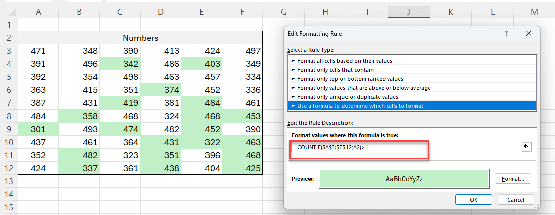
And, this checks for duplicates across the specified columns and highlights them.

12. Conclusion

Finally, in this article we have tried to explain how to highlight duplicates in Excel with formulas, different methods and tips.

In addition to basic finding duplicate features, we have also explained how to apply your formula in different scenarios and requirements. Basically, you can use conditional formatting with COUNTIF() function as the most flexible way of highlighting duplicates. Therefore, all you have to do is configure the formatting range and play with the formula, especially with the absolute and relative cell references.

To support this article, we highly recommend you to visit our Advanced Tips for Conditional Formatting article, too.

Hope you enjoy our article!

Recommended Readings:

Conditional Formatting for Pivot Table in Excel

How to Lock Cells in Excel? Prevent your cells from editing

XLOOKUP VS INDEX MATCH: Which is better and why?