How to Wrap Text in Excel? Everything about wrapping

Do you want to get into second line within the same cell in Excel workbook? Then, this is called Wrap Text, and this article will explain How to Wrap Text in Excel with examples, expert tips, possible issues, and shortcut keys.

Table Of Content

1. What’s Excel Wrap Text?
2. How to Wrap Excel Text?
3. How do I wrap Excel chart text?
4. What is the shortcut for Wrap Text?
5. Troubleshooting
6. Conclusion

1. What’s Excel Wrap Text?

Excel wrap text is basically breaking text into two or more lines in the same cell. So, it is simply writing multi-line texts in spreadsheet cells.

Actually, Excel has three main formatting options for cell text. The main choices:

• Wrap Text: This feature breaks text into multiple lines within a cell to prevent it from spilling over or being cut off.
• Shrink to Fit: This option shrinks the font to fit the cell. It’s useful but may make text too small to read.
• Overflow: If empty cells are nearby, text overflows.

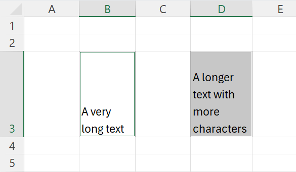
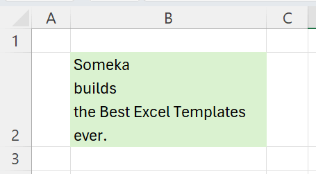
Let’s see these three different options in an example:

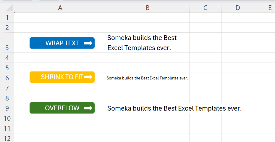
All three options have some limitations, and also benefits. Wrap text creates a better look and readability, while shrink-to-fit brings more organized and clean look.

*PRO TIP: Excel worksheet comes with overflow by default. If you want to give wrap text or shrink-to-fit, then you have to change the formatting of cell(s).

Now, we’ll see how to wrap text in Excel with examples.

2. How to Wrap Excel Text?

Wrapping is just breaking your cells into multiple lines. But, you can do this either manually or automatically. Let’s look closer to these two options.

Automated Text Wrapping

Actually, automatic wrapping is the easiest way to fit all your text in a cell. Basically, you change the formatting of the cell and Excel automatically wrap your text according to the width of your column.

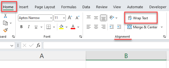
• Select cell(s) to wrap text
• From the ribbon, go to Home > Alignment > Wrap Text

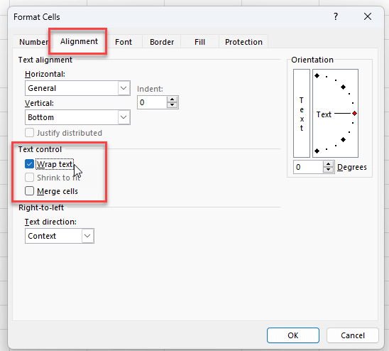
Alternatively, you can open Format Cell dialog box with CTRL+1 shortcut key, and then go to Alignment Tab and checkmark the Wrap text box under Text control settings.

So, the row height will automatically adjust to show all the text in the selected cells.

Please remember that your text will be cut from the best fit according to the column with of the cell.

If you have more than one cells at the same row with Wrap Text formatting, then the row height will adjust according to the longest text.

This is how you can easily wrap text in Excel.

But, as you can imagine, this method is easy but is hard to customize. You cannot decide on the breaking point of the text. How to do that? Let’s go to the next section.

Manually wrap text

Firstly, the manually inserting line breaks gives you more control over text wrapping. This method helps break text at specific points.

• Double-click into your target cell or press F2 to edit the cell
• Place the cursor where to break the line
• Line breaks are made with Alt + Enter

So this method give me opportunity to divide my text from different points. For example, in the below image, you can see that the same text in the same-width cells are broken from different points.

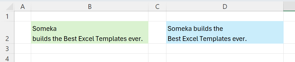
Also, you can repeat the same steps to add multiple line breaks to a cell.

*PRO TIP: If you cannot see the all lines, just double click on the row line and this will adjust the height of your rows again.

Manual vs. Automatic Wrap

Basically, the main differences between automatic and manual wrapping are control and convenience.

General-use automatic wrap text adjusts cell text automatically. However, manual wrap text allows precise control over text breaks, which is useful for structured data entries or specific formatting requirements.

Also, if you’re using Manual Wrap, you might skip the spaces between the words. This might seem like no problem from the visual side, but from the data side, this might be a big problem.

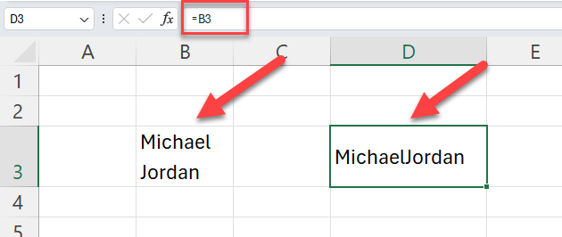
For example, in the above image, the first manually wrapped text seems like Michael Jordan, but in fact it is MichaelJordan.

3. How do I wrap Excel chart text?

If you’re working on shapes or text boxes, manual wrap text will again work. But for the axis labels on the charts, this is a bit more tricky. Even if you make the source data for the y-axis label to Wrap Text, this will not help on the chart.

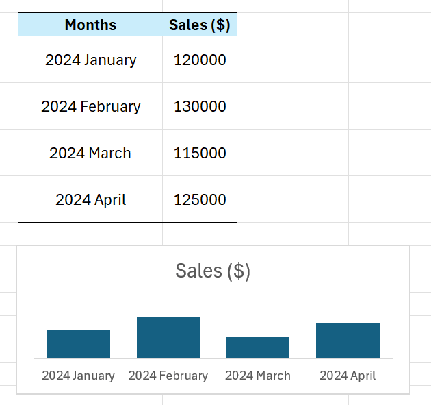
Normally, Excel adjust the lines of the axis labels automatically according to the size of your chart. But if you want to take full control over it, then the best way is to make some manipulations with the formula.

We’ll use CHAR(10) function here, which is a special character which inserts a line to the text. You can concatenate your texts with the lines using the below formula with CHAR() function:

So, this will change the data for the y-axis and will reflect to the chart y-axis.

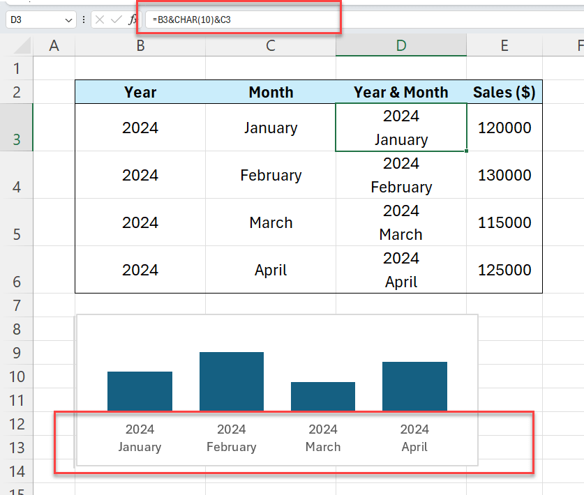
That’s how you can easily wrap text on the chart axis labels.

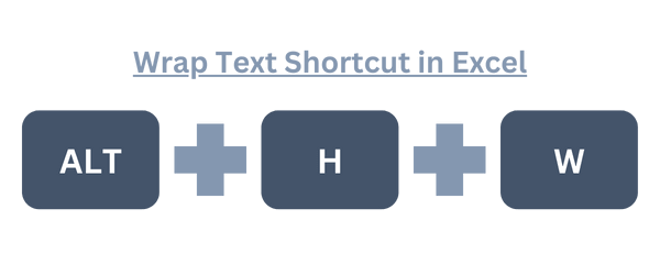
4. What is the shortcut for Wrap Text?

We can hear you asking for a more short way to add wrapping format to a cell. Sure, as every single action, Excel has also a keyboard shortcut for this feature.

After selecting the cell(s) you want to add wrapping, type Alt + H + W from your keyword.

Walla, you’re now one of those mouse-free pro users!

5. Troubleshooting

As always, you may be having some issues with wrap texting, probably because of very simple problems. Let’s check the common issues that you might be having.

Why is my text not wrapping in Excel?

Shrink to fit

Shrink to fit and Wrap text are two features against each other. In other words, you can not use these two together.

So if your text has shrink to fit feature, you simply cannot wrap text it. You should decide on one of them.

Merged Cells

The merged cells are always problematic with Excel features, and wrap text is not an exception.

If you have more than merged cells in the same row, then you might have issues with the wrap text functioning. You can re-adjust your row heights for particular cells by double-clicking on the line.

Fixed Row Height

Another very common issue preventing wrap text  is having fixed row heights in the cells. If you have manually changed the height of row, then even if you add a Wrap Text formatting to the cell afterwards, this cell will not be automatically expanded.

Here we recommend using AutoFit Row Height feature to correct this issue.

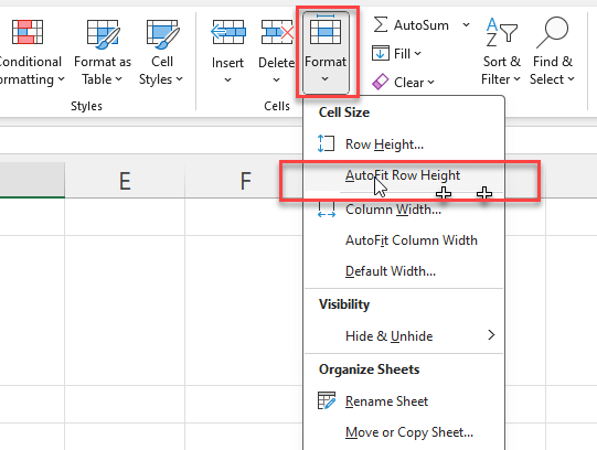
Go to Home > Format and click on AutoFit Row Height and this will fix your wrap text issue.

Horizontal Fill Alignment

Firstly, the Horizontal Fill Alignment is an option for Excel users who does not want to overflow to the adjacent cell, but also does not prefer shrink to fit option.

However, this preference is also preventing wrap text. So, if you’re having issues about wrapping your text in Excel sheet, you can check for this setting.

Open Format Cell dialog box with CTR+1 shortcut, and check the horizontal setting under the Alignment tab.

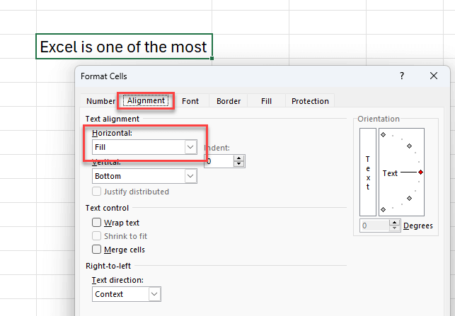
Is this is Fill option? Then, change it to another horizontal alignment again.

Already wide cell

This might seem obvious, but sometimes users might be careless about the width of the column.

Maybe your cell is already wide enough!

If this is the case, just narrow your column or add more texts to your cell. Or, just format your cell for automatic wrap text and let the excel adjust the row heights according to your text lengths.

6. Conclusion

In summary, we have try to explain how to wrap text in Excel in this article. After giving some overview on the general text control options, we have deep dive into both manual and automatic wrapping options.

Then, we have also try to explain how to wrap chart axis labels, as this might be a little tricky for some users.

Lastly, we have also underline some probably issues preventing the wrap text feature in Excel.

Thus, if you enjoy this article, stay tuned for more expert tips!

Recommended Readings:

Excel Dashboard Design: How to make impressive Excel dashboards like Someka does?

XLOOKUP VS INDEX MATCH: Which is better and why?

Excel Conditional Formatting Examples – An Advanced Approach for Power Users