How to Apply Conditional Formatting for Pivot Table in Excel?

Pivot tables and conditional formatting are two very useful features of Excel. But what about Pivot Table Conditional Formatting? In this article, we’ll explain the tips of applying conditional formatting in Excel pivot tables without having any issue.

Table Of Content

1. What’s pivot table conditional formatting?
2. How to setup conditional formatting for pivot tables?
3. Adding icons on pivot tables
4. Applying data bars to pivot tables
5. Adding pivot table color scales
6. Custom formulas for pivot table conditional formatting
7. Keeping conditional formatting in a pivot table after refresh
8. How to modify a pivot table conditional formatting rule?
9. How to delete a pivot table conditional formatting rule?
10. Conclusion

Firstly, it is important to understand that it’s a bit different to apply conditional formatting to pivot tables than the regular ranges. So, before we start, we’ll underline the main basics in order not to have problems on the road.

1. What’s pivot table conditional formatting?

So, let’s start with defining the pivot table.

A pivot table is a data summarization tool frequently used in Excel and other spreadsheet programs. It’s used to arrange and reorganize data from a large, detailed data set into a format that’s easier to understand, analyze, and report on.

Please remember that the pivot tables create dynamic ranges.

On the other hand, the conditional formatting is used to automatically apply formatting to cells in your spreadsheet based on the data they contain. So, the conditional formatting works on specific criteria.

With the regular ranges, it’s easy to apply conditional formatting. But when it comes to pivot tables, you’ll need to have dynamic formats, as pivot tables are designed to make flexible and dynamic analysis with a large data.

2. How to setup conditional formatting for pivot tables?

Applying conditional formatting to pivot tables involves both pivot table and conditional formatting knowledge. Let’s explain it with step-by-step instructions:

Step 1: Select a cell in the Values area

Firstly, you should select a cell from the column where you want to add conditional formatting.

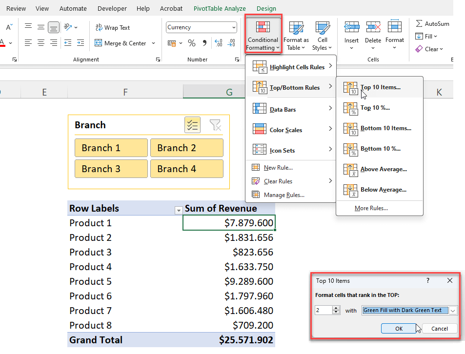
Step 2: Apply Conditional Formatting

Now go to Home > Conditional Formatting from the top menu, and configure your rules.

For example, we have a pivot table of different products and sales revenue with slicer of four different branches. And, we want to highlight top two selling products.

So we select Top/Bottom Rules from the menu and configure our settings with top number and formatting style:

So, in the example above we have used a built-in preset rule of Excel conditional formatting. But you can also use a custom one, which we’ll see later.

Step 3: Set up formatting options

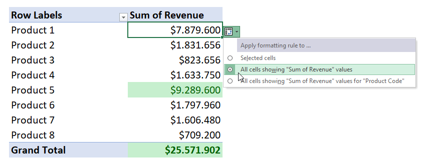
When you apply the condition formatting, you’ll find a tiny little icon called Formatting Options. So, now click on this icon.

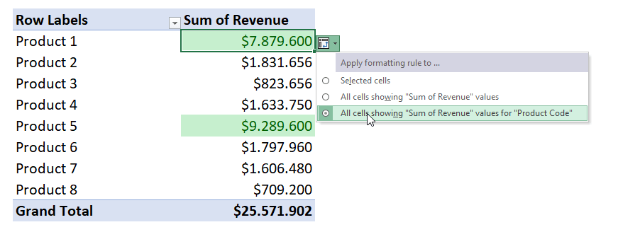
The icon will give you the options about your conditional formatting. As you see above, there are three options:

• Selected Cells: This will apply the formatting only to the cell that we have selected.
• All cells showing “Sum of Revenue” values: This option will apply the formatting to the entire column under the Sum of Revenue heading. This will include the Grand Total, too.
• All cells showing “Sum of Revenue” values for “Product Code”: This will not include the Grand Total to the formatting range.

If we select the second option, you’ll see that the formatting will be also applied to the Grand Total, which we usually do not want.

So in order to exclude Grand or Sub Totals from our range, we should select the Values for specific group of our pivot table.

But there are also some cases you want to apply the formatting to the Grand Totals. For example, if you’re analyzing a yearly change or an average, we might be also want to see formatting on the grand totals. Let’s see this example below in the icons section.

3. How to add icons to pivot table?

Icons are also preset formatting feature of Excel. So, to add icons to your pivot tables, go to Home > Conditional Formatting > Icon Sets and select the most suitable group for you.

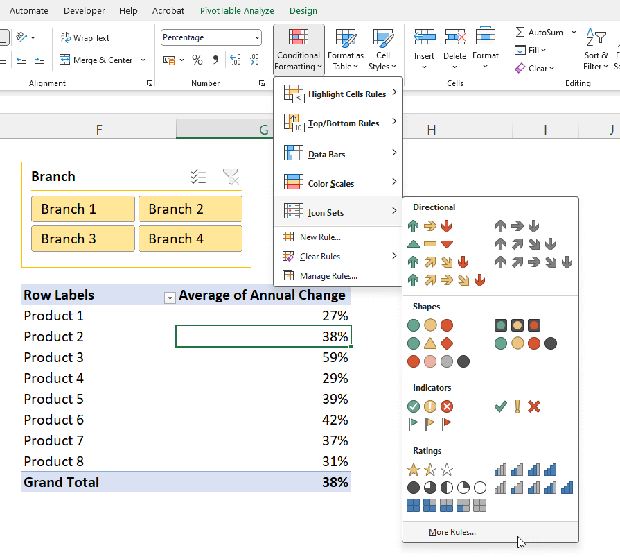
In the above image, we’re analyzing the Annual Changes in the sales of a group of Products. So we’ll also include the Grand Totals to the range:

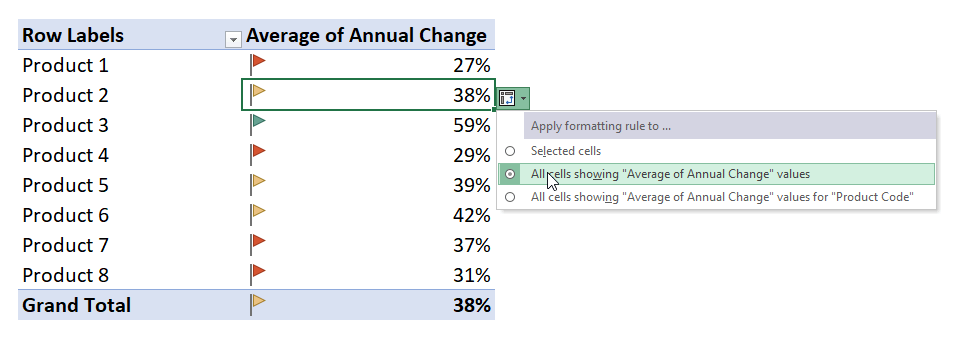
Now, we also see the iconized value of the Grand Total.

4. How to apply data bars to pivot tables?

Data bars are also very useful preset formatting tools to make quick comparisons between different values.

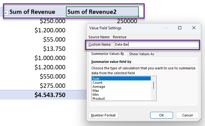
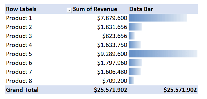
Firstly, for a more decent analysis view, we recommend to add the Value column twice to your pivot layout and give this one a different name such as Data Bar, Comparison, etc.

In the below image, we have added the Revenue heading twice to the value area and named it as Data Bar.

Secondly, go to Home > Conditional Formatting > Data Bars or open the Formatting Rule dialogue box.

Here, we will exclude the Grand Total row by selecting the third option for the applied range and then configure our styling preferences:

In the below image, we select a Gradient Fill of blue color. You can use a Solid Fill, add borders, or change the var direction according to your needs.

Thus, we recommend you not to include Grand Total or Sub Total rows in this case, as this will ruin your data bar configuration. Because your comparison will not make sense against the total row.

5. How to apply color scales to pivot table?

Color scales let you create heat maps according to the given values and are among the most common data visualization tools.

To add color scales to your pivot tables, go to Home > Conditional Formatting > Color Scales. You can select a pre-built one from the list and then change the range from the Formatting Options.

Or, you can directly add a new rule and make all the arrangements on the formatting window:

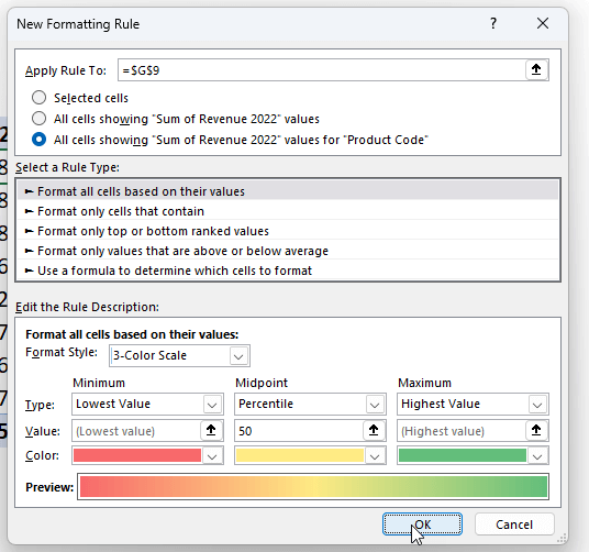
Again, be careful about selecting the range. You should apply your formatting to the all cells under the specific headings.

Then select 2-Color Scale or 3-Color Scale from the Format Style.

If you want, you can also change the colors, percentile, minimum and maximum values here.

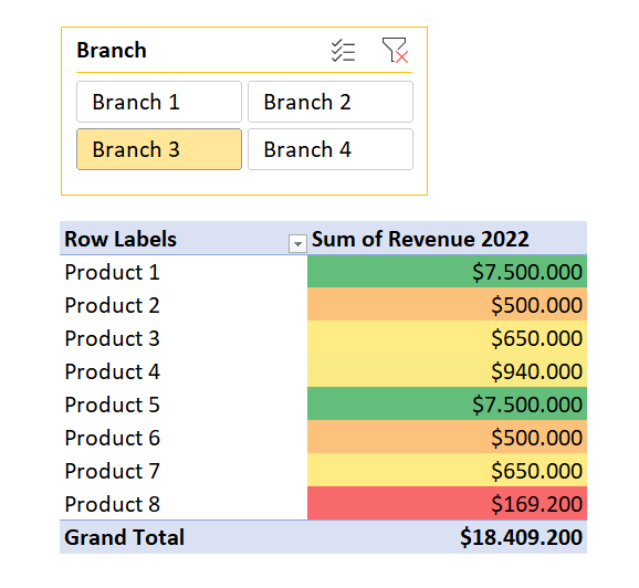
Now you have a dynamic color scale on your pivot table.

6. How to apply custom formula for pivot table conditional formatting?

In addition to built-in formatting options, you can also add custom rules to your pivot table.

Firstly, go to Home > Conditional formatting > New Rule.

Then we’ll again arrange our range to apply our formatting and set a formula-based custom rule.

For example on the above image, we have highlighted the Sales Values above $1.000k with a sales quantity of lower than 500. This is a simple example of custom rules in pivot table conditional formatting.

7. Can I keep conditional formatting in a pivot table after refresh?

Yes, of course you can.

If you apply the conditional formatting on the defined pivot table ranges, not the regular cell ranges or columns or rows, you will not lose your formatting rules.

But if you select the whole column and apply the formatting rules, then:

• It will apply the conditional formatting not only to the pivot table, but also to the entire column.
• When you use the filters or slicers, you’ll lose the formatting.
• When you refresh your file, your formatting will be gone.
• If you change the layout of your pivot table from the side menu, you cannot keep your conditional formatting.

For example, in the above examples we set our formatting to the pivot ranges, not the regular cell references. So we have a dynamic formatting. Even we change the slicer preferences, our rule still continues to populate:

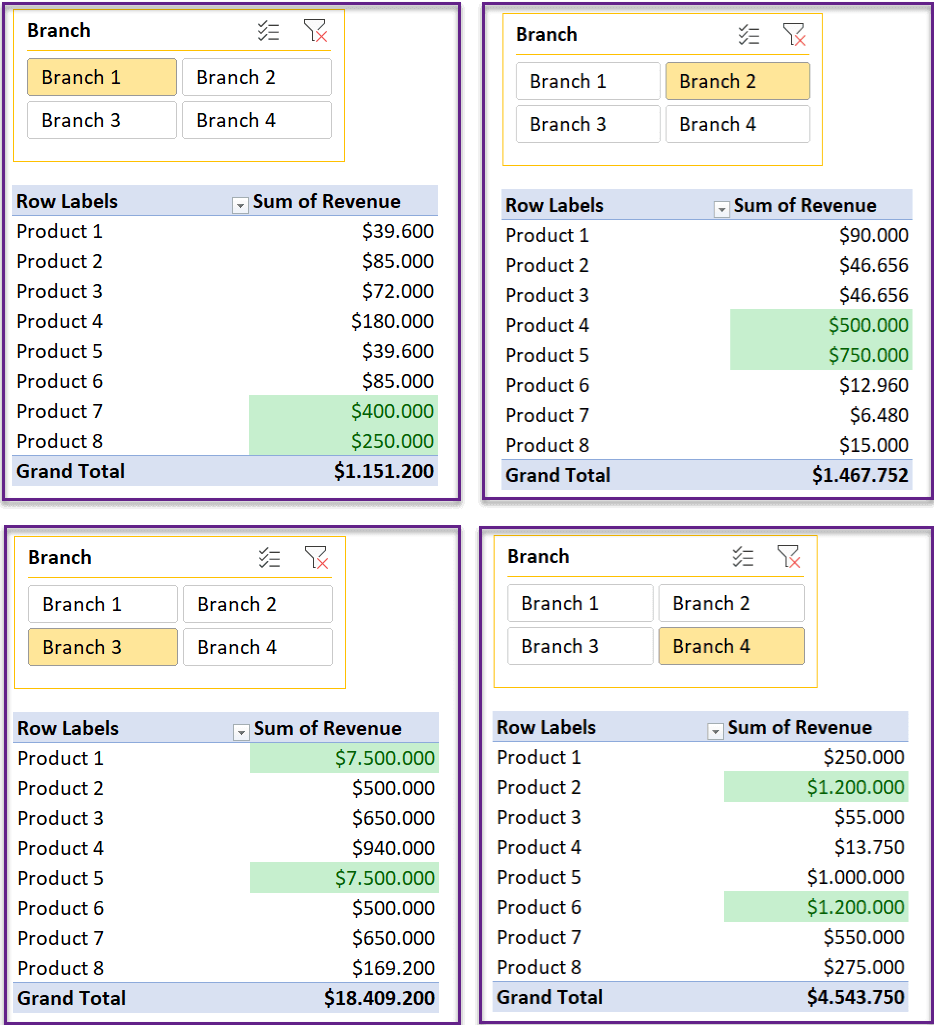
We change the slicers, and the top 2 selling product highlights updates accordingly.

This is the mystery of dynamic formats!

What if I remove the pivot range with a conditional formatting from the layout?

If you remove a heading from your pivot table, then the conditional formatting rule applying to that heading will be also removed.

So, if you wat to make different dynamic analysis, you can always make a copy of your pivot table sheet in order not to mass up the previous sheet.

8. How to modify a pivot table conditional formatting rule?

You can always edit your rules from the Conditional Formatting dialog box.

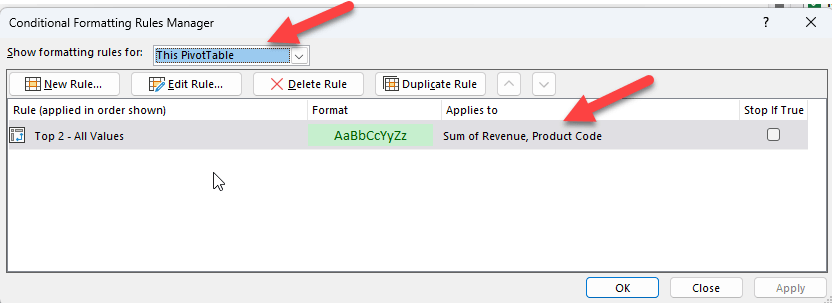
So, go to Home > Conditional Formatting > Manage rules and after selecting the relevant rule, click Edit Rule tab.

You can change your range, style, and criteria here to modify your rules for the formatting.

9. How to delete a pivot table conditional formatting rule?

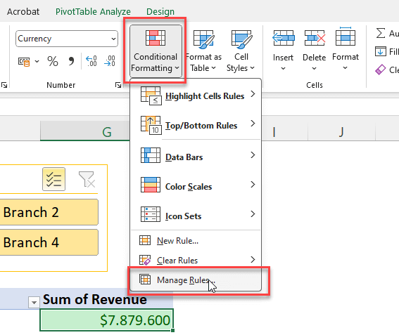
To delete a pivot table conditional formatting rule, click on any cell on the pivot and go to Home > Conditional Formatting > Clear Rules and Clear Rules from This Pivot Table.

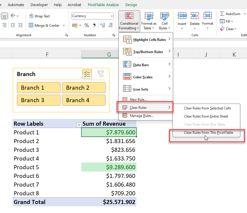
This will clear all the rules in the selected pivot table. If you want to clear one of the many rules, then you will go to Manage Rules and click on the small Delete Rule button on the Conditional Formatting Rule Manager.

10. Conclusion

In summary, we have explained how to set up conditional formatting rules in pivot tables, including data bars, icon sets, color scales as well as custom criteria.

For the pivot tables, the key point is defining the ranges to apply your formatting rules. You should always use the pivot table ranges, not the regular cell references. In this way, you will keep your formatting with slicers, filters, refresh, layout changes or even data changes.

Hope this post will help you to make better data analysis presentations!

Recommended Readings:

Conditional Formatting in Google Sheets: Comprehensive Guide with Examples

Can Excel Analyze Data?

How to make your Excel files look MUCH better?