How to Strikethrough in Excel? Easy Ways and Advanced Tips

Strikethrough formatting lets you show that a task is done, that data is no longer valid, or that information should no longer be considered. But how to add this strikethrough in Excel? Here’s a complete guide for you.

Table Of Content

1. How to strikethrough in excel?
2. Strikethrough Shortcut in Excel
3. Partial Formatting with Strikethrough
4. Strikethrough with Conditional Formatting
5. How to Automatize Strikethrough Formatting?
6. Conclusion

1. How to strikethrough in excel?

You can easily add strikethrough formatting in Excel with some basic steps.

Step 1: Select the relevant cell(s)

Firstly, you should choose the cell or cells that you want to change. So, either click on a single cell or click and drag your mouse over several cells to select them all.

Step 2: Click on the Format Cells box

Secondly, you’ll open the format cell dialogue box. Therefore, you have three options: 1. Ribbon, 2. Right-click menu, 3. CTRL+1 Shortcut.

• Ribbon Method: On the Excel ribbon, go to Home > Cells > Format Cells.

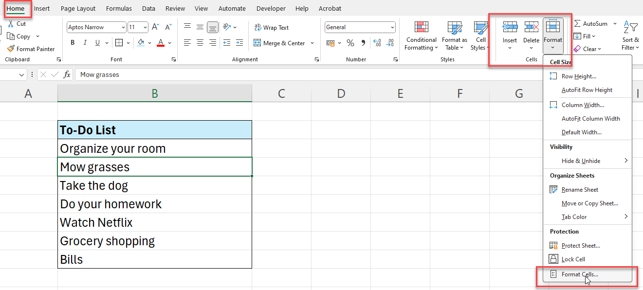
• Right-Click: Right-click on the cell(s) you want to change and select “Format Cells” from the menu that appears.
• Shortcut on Keyboard: The Format Cells dialogue box will quickly appear when you press Ctrl + 1.

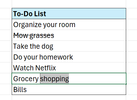
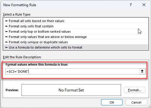
Step 3: Check the box next to Strikethrough

Lastly, on the Format Cell dialogue box, under the Fonts tab you can find Strikethrough checkbox under the effects.

So, once you’ve chosen this option, click “OK” to give the selected cells the strikethrough look.

2. Strikethrough Shortcut in Excel

As many actions, strikethrough has also a shortcut in excel.

After selecting the cell or range you want to strikethrough, just click on CTRL+5 on your keyboard. This will put a line on the text directly.

3. Partial Formatting with Strikethrough in Excel

The above methods strikethrough the entire text in a particular cell. But, there are times when you might only want to strikethrough a small part of the text in a cell and not the whole thing.

That’s also possible:

• First, dive into the cell with double-click it or press F2
• Secondly, select the part you want to strike through text in a cell

• Thirdly, open Format Cell window with CTRL 1
• Then, go to Font > Effects > Strikethrough
• Lastly, click OK

This method lets you keep the formatting of your text flexible, so you can highlight or underline certain parts of the cell content.

4. Strikethrough with Conditional Formatting

With conditional formatting in Excel, you can change the way something looks based on certain conditions. This is helpful for strikethrough formatting because it can do it automatically based on the state of your data.

For example, we want to strikethrough the tasks that are DONE.

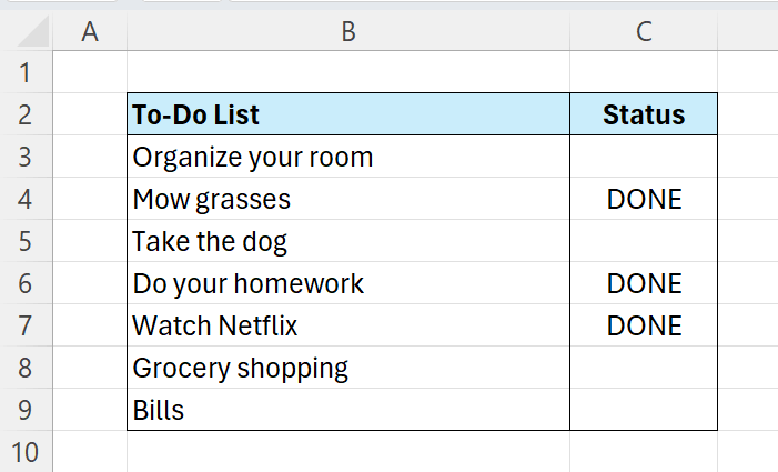
Firstly, select your tasks range, and go to Home > Conditional Formatting > New Rule.

We’ll use a formula to manage our rule.

This formula says that if the adjacent cell (here it’s in the C column) is “DONE”, strikethrough the selected range (in this case it is in the B column).

Lastly, checkmark the Strikethrough option on the formatting window.

Now you have created a dynamic conditional formatting for your tasks.

You can also use strikethrough option with Excel checkboxes.

In this time, you’ll build your conditional formatting rule formula to check if the adjacent cell is TRUE or not.

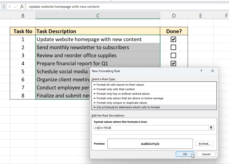
This will create a checklist where the item turns stroked when the checkbox is marked.

5. How to Automatize Strikethrough Formatting?

If you’re using this strikethrough formatting feature too often, you might add a button to add strikethrough texts at one click.

You can add such buttons with macro, Excel Ribbon or Quick Access Toolbar.

a. Strikethrough button with a macro

You can use strikethrough formatting with just one click if you make a macro.

• Open your VBA editor with Alt+F11
• Go to Insert > Module to add a new module
• Add the below code and close your editor

Sub ApplyStrikethrough()
Selection.Font.Strikethrough = Not Selection.Font.Strikethrough
End Sub

• Insert a shape as your button and name it
• Right click on the shape and select Assign macro from the menu
• Select your strikethrough macro and click ok.

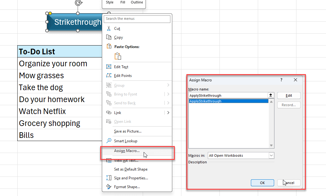
Now when you click on this button, the click cell or range will have strikethrough formatting.

b. Adding a strikethrough button to your Excel Ribbon

You can add a button to your Excel Ribbon for the strikethrough macro to make it even easier to use:

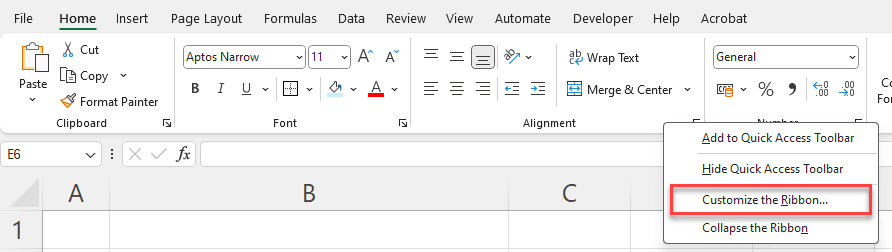
• Right click any spot on your ribbon
• Click Customize Ribbon

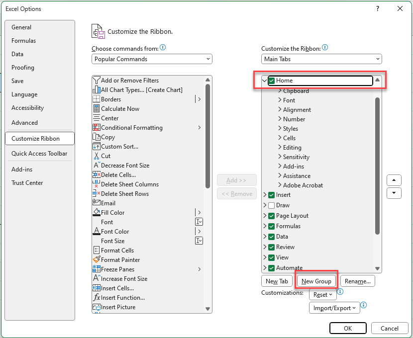
Next, on the Excel Options window, choose a tab (in the below example the home tab is selected) and click “New Group”

Then find the strikethrough command under the commands list and click Add.

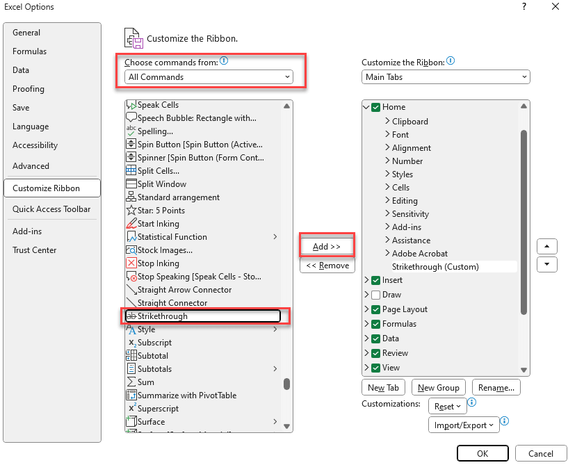
And click OK to save your changes. So, now you have a direct access from your ribbon.

c. Adding a Strikethrough button to Quick Access Toolbar

Again open your Excel Options window. Then, go to Quick Access Toolbar from the left-side menu. Secondly, find the Strikethrough command under the list and click on add.

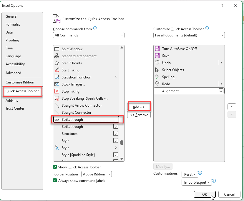
Lastly, click on OK and save this.

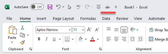
Now you have a strikethrough button on your Quick Access Toolbar.

That’s all for the adding automatization buttons for Excel strikethrough formatting.

6. Conclusion

Finally, the strikethrough is a flexible formatting tool in Excel that can help you better manage and arrange your data.

Thus, we have tried to explain you how to strikethrough your entire or partial text in a cell or in a range. Then, we have also given you the strikethrough shortcut so that you can apply it without using your mouse. Finally, we have also given some advanced tips on adding direct buttons for strikethrough command.

So, hope you enjoy our article on Strikethrough in Excel!

Recommended Readings:

How to use XLOOKUP Multiple Criteria in Excel?

Complete List of Things You Can Do With Excel

How to fix #VALUE! Error in Excel?