SUMIFS Function in Google Sheets

We collected all the fundamentals for the SUMIFS Google Sheets function below and presented you with different examples to demonstrate! So, read now and learn how to use SUMIFS in Google Spreadsheets now!

What is Sumifs function in Google Sheets?

Sumifs is a built-in function in Google Sheets that helps you to sum up your database based on multiple criteria.

How to use Sumifs in Google Sheets?

If you have a database and you want to use the sumifs function in Google Sheets, this post will help you understand how to use the function.

Firstly, let’s check the structure of the sumifs formula Google Sheets:

=SUMIFS (sum range, criteria_range1, criterion1, [criteria_range2, …], [criterion2, …])
sum range	Select the range that you want to sum.
criteria_range1	This is the range for the first criterion.
criterion1	This is the summing criteria for the first criteria range.
criteria_range2	This is the range for the second criterion.
Criterion2	This is the summing criteria for the second criteria range.

 

Let’s check a sumifs Google Sheets example:

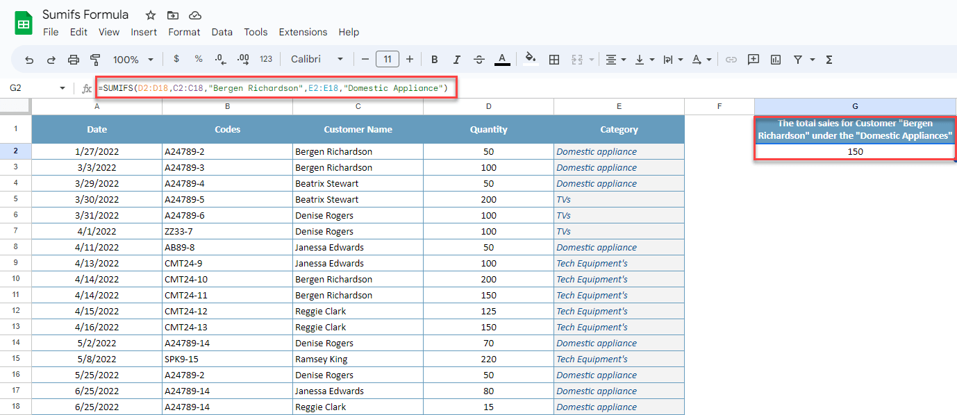
Suppose we want to see the total sales for Customer “Bergen Richardson” under the “Home Appliances” Category.

1-Firstly, we need to select the sum range which is the Quantity column

2-Secondly, now we need to choose the first criteria range which is Customer Name Column

3-Thirdly, write the Criteria for the first criteria range

4- Then, we will choose the second criteria range which is Category

5-Lastly, we will write the second criteria for the second criteria range

Now we are ready to see the total sales based on multiple criteria that we set above.

Let us check how to use google sheets sumifs multiple criteria using the date on the same example:

1- Firstly, let’s assume that we want to see the total sales in April

Again we will choose the sum range which is the total sales column

2- Now select the date column for the first criteria

3- After that, write the first criteria which is the date.

The date should be higher than or equal to the 1st of April 2022.

4- Again, we will select the date column.

5- Finally, we will write less than or equal to formula for the 30th of April 2022.

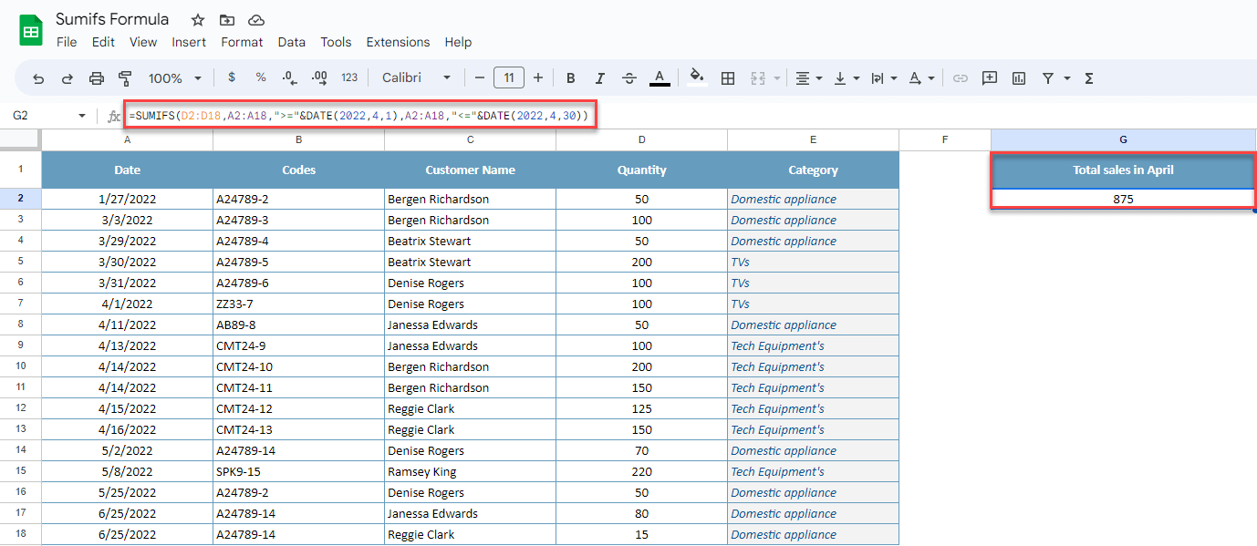
Now we know that we sold 875 products in April!

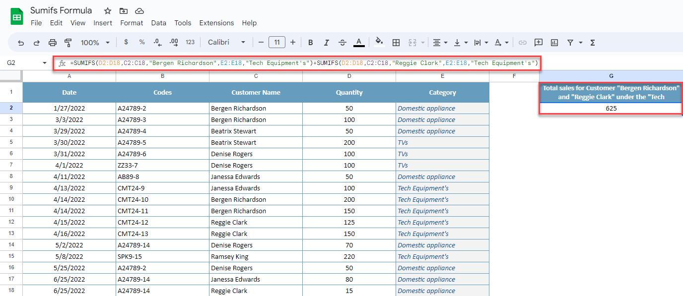
Sumifs Formula in Google Sheets Using OR Criteria

So far, all Sumif conditions, which we showed, used an AND logic. In some situations, OR logic is also needed. So, let’s check how to use sumifs in google sheets with OR logic with the same database.

For example, we want to see the total sales for Customers “Bergen Richardson” and “Reggie Clark” under the “Tech Equipment’s” Category.

The best way to use “or” criteria with sumifs function is using more than one sumifs in the cell.

Firstly, the formula for “Bergen Richardson” and “Tech Equipment’s”

And the second formula for Reggie Clark and “Tech Equipment’s”

So, the final formula will be as follows:

 

Using a SUMIFS Function with Logical Operators

First, we need to define logical expressions. You can see the logical expressions on the table below.

Greater than (>)

Less than (<)

Greater than or equal to (>=)

Less than or equal to (<=)

Equal to (=)

Not equal to (<>)

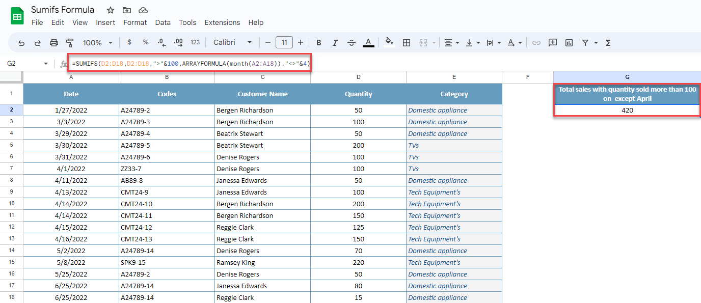
So, now we can find Total sales with quantity sold more than 100 on except April.

1- Firstly, we need to choose the sum range:

2- Secondly, we need to choose criteria for quantity.

3- Now, we will use a logical expression which is Greater than (>) and “&” expressions.

4- Then, we need to choose the date column to check the month.

5- Finally, we will add Not equal to (<>) with “&” expressions.