VLOOKUP Google Sheets Function and Alternatives

VLOOKUP in google sheets works very similarly to its Excel brother.

There are 4 inputs: searched value, the range where we are searching the value, the column number of the result, and the is_sorted parameter which means that it searches for the exact or not exact match.

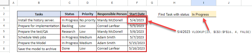
The range in this case has to begin with the column that contains our searched value. In this case status “In Progress”. The return value comes from column number 4 within the range, so it will give us the first date where the status is equal to “In Progress”

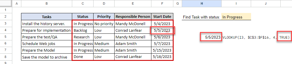
If however, I change the last parameters to TRUE the result will be completely different. Vlookup Google Sheets function will give us the next value after the first match.

Can we get multiple results using VLOOKUP?

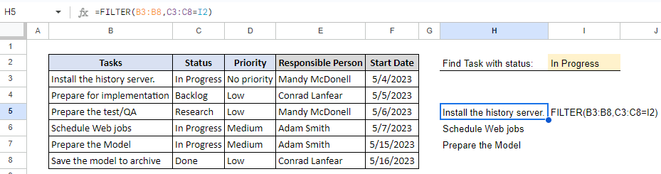
In our example, we have 3 tasks where the status is equal to “In Progress”. Basic Vlookup in Google Sheets does not allow us to get all those results.

But we can easily get the result using another formula instead of Vlookup in Google Sheets: the FILTER formula.

Let’s say I wanted to see all Task titles where priority is equal to what I can find in cell “I2”.

In the first parameter, I give the range that will be filtered and in the next parameters, I give my conditions:

In this case, I filter the range of cells B3:B8 and my condition is if any of the cells from range C3:C8 is equal to “In Progress”.

I can modify the formula and get a result of a few columns, for example Tasks, Status & Priority where my condition checks the Responsible person:

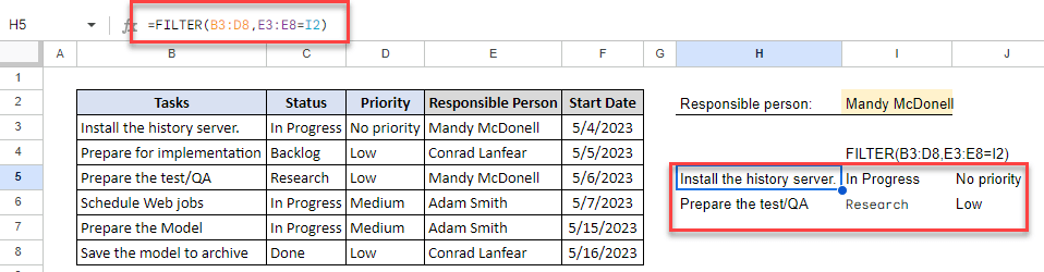
We need to make sure the range where we will get the result is empty and does not contain any values or formulas. Otherwise, we will get a reference error.

If we want to combine results from different columns in one column we can always use a “&” to connect results as strings:

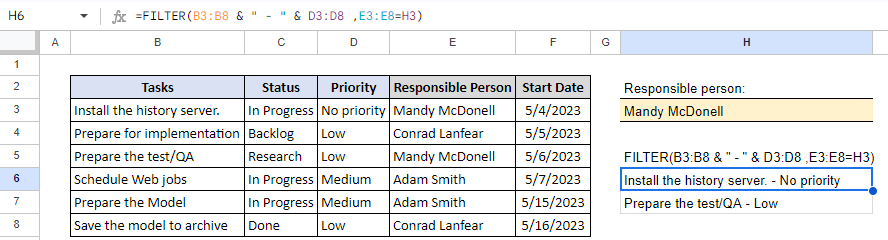
In the above example, we combined values from columns B and D and connected them into one result.

We can use as many criteria check as we need. If we want to see all tasks that are before the 15th of May and have priority Low it will be as simple as the previous examples. Here we have directly written the condition so they are not related to any filter like before.

As you can see, you can use FILTER function as an alternative to VLOOKUP in Google Sheets.

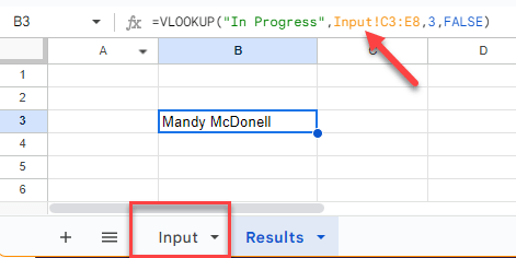
Is it possible to use Vlookup to get data from other sheets?

Yes, Google Sheets allows you to use all the formulas with a current sheet, another tab, or even a completely different file. So, you can use Vlookup in Google Sheets for this purpose. Below, the input table is still the same but it is in the sheet named “Input”. The only change I need to include is the name followed by “!”.

To use data in other Google Sheets files I need to copy the URL address of the input file:

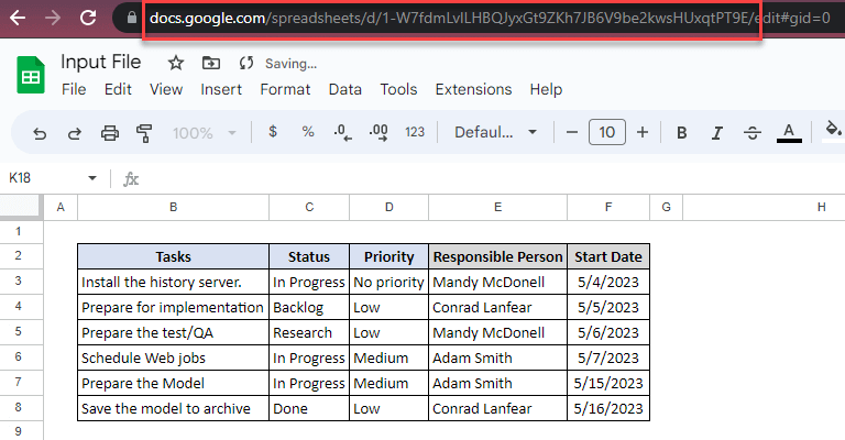
Then import directly to my new file using the IMPORTRANGE formula.

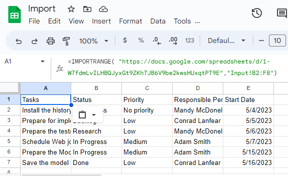
Now we can use our imported data as we used it before. Create a VLOOPUP formula in a separate cell. We can also use the formula directly by taking the import range as our range inside the formula.

Let’s also see this formula in our instructional tutorial video:

In summary, the VLOOKUP and FILTER formulas are both powerful functions in Google Sheets. They help users find specific data and filter results based on specific conditions.

VLOOKUP has a bit more limitations but you can use the FILTER formula as an alternative to overcome this issue. Additionally, by using the IMPORTRANGE formula, we can always easily access and use data from other sheets or workbooks. Those and other functions can help easily analyze data in Google Sheets.

You can also use other functions in exchange of basic Vlookup in Google Sheets. INDEX combined with the MATCH function is also usable. You can also check out the QUERY function, which is not available in Excel.