How to use XLOOKUP Multiple Criteria in Excel? Guide with 3 Easy Options
Today, we’ll explain expert tips to use XLOOKUP function in Excel with multiple criteria. As one of the newest functions of Excel, XLOOKUP helps users to look for a certain value with criteria-based conditions. Now, this article will explore XLOOKUP Multiple Criteria with three easy ways.
Table Of Content
1. What’s XLOOKUP Function in Excel?
2. How to use XLOOKUP Multiple Criteria?
- Option 1: Using Boolean logic to create arrays
- Option 2: Using Concatenation
- Option 3: Using Logical Operators
3. Example to use XLOOKUP with Multiple Criteria in Excel
Let’s start!
1. What’s XLOOKUP Function in Excel?
As of 2020, Microsoft added the XLOOKUP function to Excel. Actually, it is a more up-to-date version of older lookup functions like VLOOKUP, HLOOKUP, and even the flexible INDEX and MATCH combination.
Many of the problems with the older functions have been fixed in this one, which also makes searching and getting data from an array.
First, let’s see how this Xlookup function works. The syntax for XLOOKUP is simple:
Let’s look closer to the required parameters of this function:
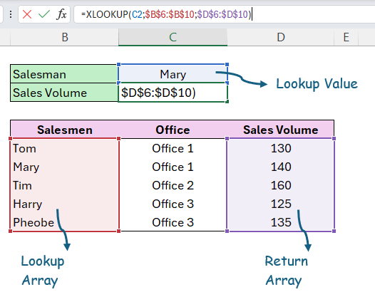
- Lookup_value: The value to search for
- lookup_array: The array or range to search
- return_array: The array or range to return
As the other parameters are optional, we’ll keep it simple now and go with the required ones.
So, XLOOKUP is great because it can be used in many ways. Firstly, it can return a value either horizontally or vertically. Also, you can use a default value if the lookup value doesn’t exist. This makes it less likely that your results will be error.
Lastly, it’s also very powerful when you use it with other functions or when working with complex data structures because it can handle arrays.
Now we’ll see how we can solve complex lookups with more than one criteria.

2. How to use XLOOKUP Multiple Criteria?
When working with big sets of data, you might need to use more than one criterion to make sure that the results of a lookup operation are correct.
We’ll check the most common three ways to lookup for specific values according to multiple criteria
Option 1: Using Boolean logic to create arrays
Boolean logic is simply the basic AND and OR conditions. You can link your criteria with AND and OR functions to meet a set of conditions.
Basically, you use a set of criteria that together produce a list of TRUE and FALSE values. In this case, you would use an array formula to combine the two conditions so that you can find data that meets both of them.
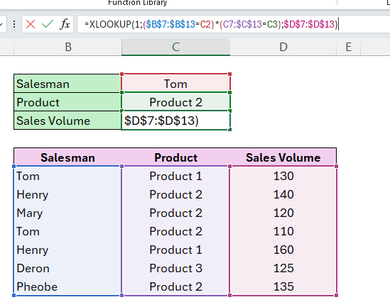
In the below example, we are looking for the sales volume of a particular salesman for a particular product. So, we have two criteria: 1. Salesman, 2. Product
So let’s make it step-by-step instructions:
Step 1: Define your criteria arrays and criteria values
Firstly, we should define our criteria ranges and criteria values. This is the main logic of our search.
Step 2: Define your return array
Secondly, we’ll define the range where we are looking for a value.
Step 3: Write your XLOOKUP formula
Your formula will search for 1 (TRUE) in the lookup array (multiplication of your multiple criteria) in the return array.
That’s all!
Option 2: Using Concatenation
Secondly, we can put together several criteria into a single lookup value with concatenation. This method works best when your criteria cover more than one column but are easy to combine into a single identifier.
Let’s apply this to our above example.

Here, we have combine our look up value with an “&” concatenator. Then, we have also concatanate our criteria arrays.
This might be the simplest way of using XLOOKUP Multiple Criteria, but you should be careful about the orders of the values. Because if the orders of the values does not match the orders of your criteria arrays, this will not give you the correct solution.
Option 3: Using Logical Operators
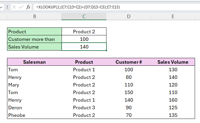
Lastly, you can use logical operators in Excel XLOOKUP function to meet multiple criteria. Basically, you can set a range or certain conditions that must be met with operators like >=, <=, >, <, and <>.
This formula uses a logical OR (shown by +) to find entries where either “Product 2” is the product or the value in column B is greater than 100. It then returns the value from the Sales Volume column that matches that entry.
So, each of these methods is a strong way to use XLOOKUP to its fullest when working with multiple criteria. Then, you should pick the one that works best with your data structure and the level of difficulty of the criteria you are working with.
3. Example to use XLOOKUP with Multiple Criteria in Excel
Now let’s make a complex example to use Excel XLOOKUP function to meet many criteria at the same time.
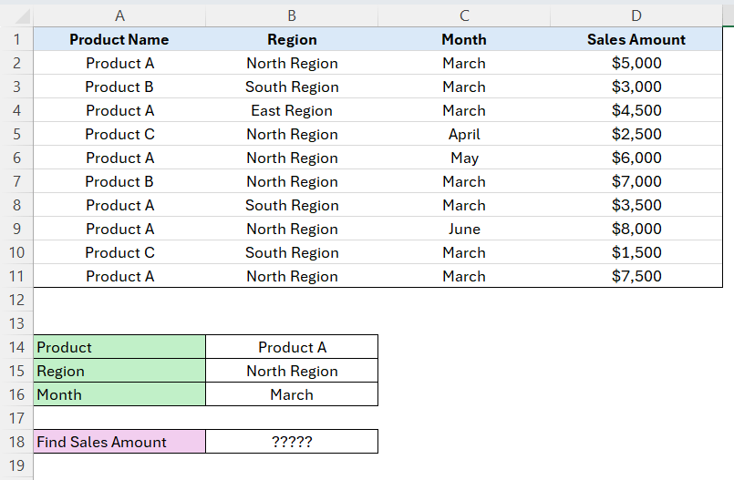
We suppose we have a dataset with sales data, and we want to find out how many of a certain product were sold in a certain area during a certain month. To do this, this example will show you how to use XLOOKUP with more than one condition.
Dataset:
- Column A: Product Name
- Column B: Region
- Column C: Month
- Column D: Sales Amount
Task:
Find the number of “Product A” sales in the “North Region” during “March.
Let’s use the concatenation method to solve this problem.
- Firstly, we have concatenated the lookup values.
- Secondly, we have concatenated the lookup arrays.
- Lastly, we have added the return array.
Here’s the solution:
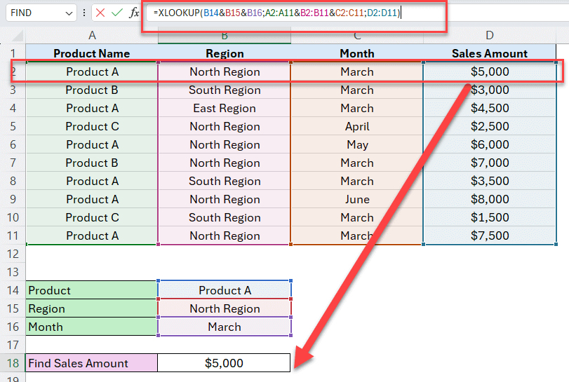
This method works really well when data needs to be matched across multiple columns, and it makes sure that the exact set of criteria is met.
Pros:
- It’s very accurate at getting the right data because it needs an exact match of the concatenated string.
- Lowers the chance of mistakes that could happen because of criteria that are duplicated or overlap in different columns.
Cons:
- Concatenation needs to be precise and well-managed, which can make it hard to do when there are more criteria or larger datasets.
- Processing strings that have been joined together might slow down operations that involve very large arrays.

4. Final Words for XLOOKUP Multiple Criteria
Learning how to use XLOOKUP with multiple criteria and its alternatives, such as INDEX and MATCH, is necessary for anyone who wants to get the most out of Excel for data analysis. These tools can help you whether you need to manage large datasets, do complex searches, or just make your workflows more efficient.
Key Takeaways:
- XLOOKUP is a flexible function that makes many tasks easier that were hard to do with older lookup functions like VLOOKUP and HLOOKUP.
- With XLOOKUP function, you can handle multiple criteria using Boolean logic, concatenation, and logical operators,.
- Even though INDEX and MATCH are older functions, they can still be used as a backup, especially when you’re using an older Excel version.
As you work with Excel, keep in mind that the goal is not just to find data, but also to understand it and use accurate analyses to make decisions.
Hope you enjoy our article!
Recommended Readings:
Excel Dashboard Design: How to make impressive Excel dashboards like Someka does?
How to Prevent and Solve Data Discrepancy Issues in Excel?
Excel Goal Seek Function Guide: Definition, How-to Steps and Examples
Related Posts