How to Use INDEX MATCH in Google Sheets

Index match Google Sheets function is a powerful function in Google Sheets that allows you to look up a value in a table based on specific criteria. It is often used as an alternative to VLOOKUP, which can be limited in its capabilities. In this blog post, we will explore what index match is, how it works, and how you can use it in Google Sheets.

What is Index Match Google Sheets Formula?

Index match is a formula in Google Sheets that combines the INDEX and MATCH functions to look up a value in a table based on particular criteria. The INDEX function returns the value of a cell in a table based on a row and column number, while the MATCH function returns the position of a specific value in a range. By combining these two functions, you can look up a value in a table based on certain criteria, such as a unique identifier.

How Does Index Match Google Sheets Formula Work?

The index match formula works in three steps:

1. Identify the column you want to return the value from
2. Use the match function to find the position of the value you want to lookup based on specific criteria
3. Use the index function to return the value from the identified column at the position found by the match function

Here’s an example:

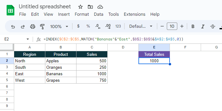
Suppose you have a table that contains sales data for different regions and products, as shown below:

You want to look up the sales of Bananas in the East region. Here’s how you can use index match to do it:

Identify the column you want to return the value from. In this case, we want to return the sales column.

Use the match function to find the position of the value you want to look up. We want to match the region and product. The formula would look like this:

This formula concatenates the region and product and matches it against the concatenated values in the table.

Use the index function to return the value from the identified column at the position found by the match function. The formula would look like this:

This formula returns the value in the sales column at the position found by the MATCH function.

Its Benefits

There are several benefits to using index match over VLOOKUP. Here are a few:

• Greater flexibility: Index match allows you to find a value based on any criteria, not just the leftmost column as in VLOOKUP.
• Easier to use with dynamic ranges: Index match can handle dynamic ranges, while VLOOKUP cannot.
• Improved performance: Index match can be faster than VLOOKUP, especially with large datasets.

Conclusion

INDEX MATCH is a powerful function in Google Sheets that can help you look up a value in a table based on certain criteria. By combining the INDEX and MATCH functions, you can create a formula that is more flexible and powerful than VLOOKUP. Remember to identify the column you want to return the value from, use the match function to find the position