How to Use SUMIF in Google Sheets

SUMIF in Google Sheets works pretty similar to SUMIF function in Excel. However, the features in Google Sheets may add different properties and opportunities to the SUMIF formula in Google Sheets. Let’s look at it from the beginning!

SUMIF Formula in Google Sheets

The basic syntax of the SUMIF is written like below:

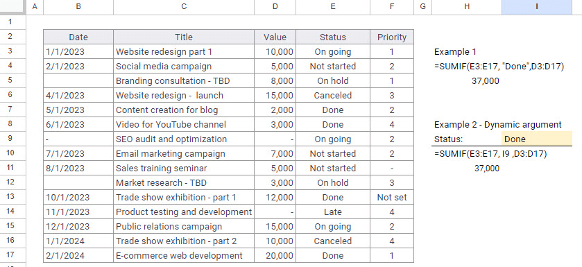
The formula takes 3 arguments. The first argument is the range where we check the condition. Secondly, you will write the condition. So, that means we are checking if any of the values, within range A1:A10, is higher than 5. Then, the third argument comes which is the sum of corresponding values from the range B1:B10.

You can use the formula directly with hardcoded conditions like in example #1. However, we can also take them from another cell as it is shown in example #2. The results are the same, but we can easily add the dropdown list to the status filter. In the end, the final result will automatically update itself with the change of the Status condition coming from Cell I9.

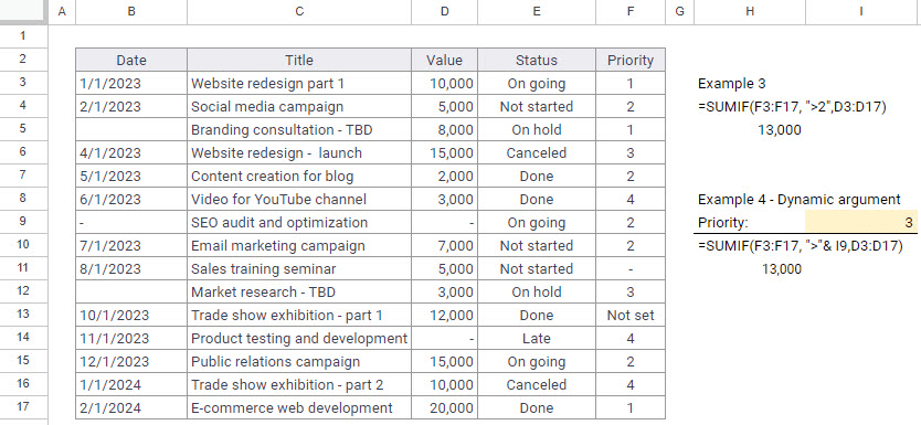
What if we want to extend our condition from a basic “if equals to” to some more dynamic solutions? Then, we have few options in SUMIF functions in Google Sheets.

In case of numbers or date-related conditions we can use:

• “>” – greater than (“>=” – greater or equal)
• “<” – smaller than (“<=” – smaller or equal forms.

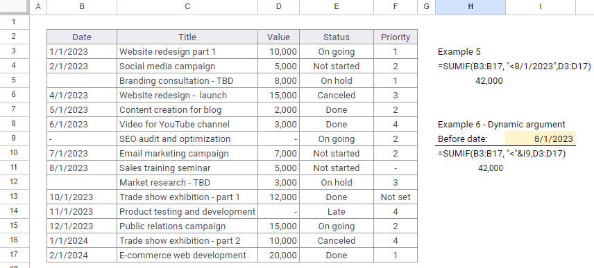
The next 4 examples are showing the syntax of using those connectors with hardcoded values and dynamic arguments. Examples #3 and #4 show the number-related conditions while examples #5 and #6 date-related formulas. In the case of dynamic argument, we need to connect the condition by using  “<” or “&” and the cell where our dynamic argument comes from.

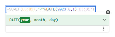
In example #5, the condition is “<8/1/2023”. However, if you want to stay safe with the date format in the SUMIF Google Sheets formula, make sure that the argument takes the correct date. So, the better solution is to use the DATE formula and wire the condition using the Date function. Thus, you can make sure that your date format is correct and days are not mixed with months.

Text Conditions in SUMIF Formula

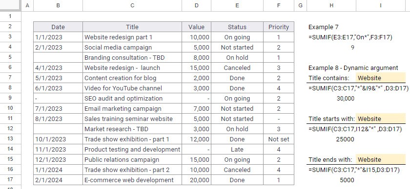
In cases of text-related conditions, we can always use the “*” in SUMIF Google Sheets formula. Asterisk (*) inside the condition allows us to match all the inputs that contain partial text. In example #8, you can see the usage of the “*” in 3 ways.

If you leave the asterisk only on the left side of the condition, that means the formula will search for all the matches where the title ends with “website”. If the “*” is on the both sides of the condition the SUMIF Google Sheets formula will search any title that contains the word “website” no matter what is before or after.

Example 10 – OR logic, when we want to sum some of the conditions. In this case, I want to sum the value of all the project parts that have no priority. In the data table, Priority considered as not set can be understood in a few ways: The cell might be empty or have values equal to “-” or “Not set”. This is why I have to create 3 separate SUMIF formulas and simply add them.

Don’t forget to check our tutorial video to learn more about this function:

In conclusion, the SUMIF formula in Google Sheets is a powerful tool for calculating and summarizing data based on certain conditions. With its simple syntax, we can easily handle a lot of dynamic conditions. We can use number or date-related conditions with the connectors “>”, “>=”, “<”, and “<=”, and text-related conditions with the star symbol “*”. You can combine it with the OR logic to sum the values of multiple conditions. Furthermore, you can use it together with other functions that Google Sheets offers. if you found the topic interesting I would recommend checking out other blog posts on SUMIFS and COUNTIF functions.